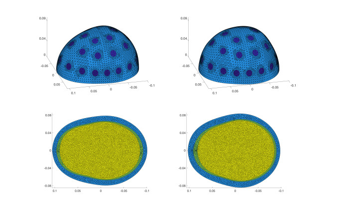
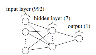
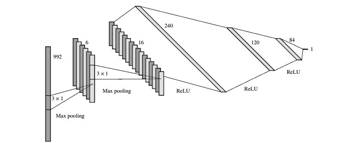
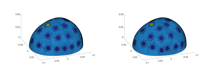
We consider the problem of the detection of brain hemorrhages from three-dimensional (3D) electrical impedance tomography (EIT) measurements. This is a condition requiring urgent treatment for which EIT might provide a portable and quick diagnosis. We employ two neural network architectures - a fully connected and a convolutional one - for the classification of hemorrhagic and ischemic strokes. The networks are trained on a dataset with $ 40\, 000 $ samples of synthetic electrode measurements generated with the complete electrode model on realistic heads with a 3-layer structure. We consider changes in head anatomy and layers, electrode position, measurement noise and conductivity values. We then test the networks on several datasets of unseen EIT data, with more complex stroke modeling (different shapes and volumes), higher levels of noise and different amounts of electrode misplacement. On most test datasets we achieve $ \geq 90\% $ average accuracy with fully connected neural networks, while the convolutional ones display an average accuracy $ \geq 80\% $. Despite the use of simple neural network architectures, the results obtained are very promising and motivate the applications of EIT-based classification methods on real phantoms and ultimately on human patients.
Citation: Valentina Candiani, Matteo Santacesaria. Neural networks for classification of strokes in electrical impedance tomography on a 3D head model[J]. Mathematics in Engineering, 2022, 4(4): 1-22. doi: 10.3934/mine.2022029
We consider the problem of the detection of brain hemorrhages from three-dimensional (3D) electrical impedance tomography (EIT) measurements. This is a condition requiring urgent treatment for which EIT might provide a portable and quick diagnosis. We employ two neural network architectures - a fully connected and a convolutional one - for the classification of hemorrhagic and ischemic strokes. The networks are trained on a dataset with $ 40\, 000 $ samples of synthetic electrode measurements generated with the complete electrode model on realistic heads with a 3-layer structure. We consider changes in head anatomy and layers, electrode position, measurement noise and conductivity values. We then test the networks on several datasets of unseen EIT data, with more complex stroke modeling (different shapes and volumes), higher levels of noise and different amounts of electrode misplacement. On most test datasets we achieve $ \geq 90\% $ average accuracy with fully connected neural networks, while the convolutional ones display an average accuracy $ \geq 80\% $. Despite the use of simple neural network architectures, the results obtained are very promising and motivate the applications of EIT-based classification methods on real phantoms and ultimately on human patients.

| [1] |
L. Borcea, Electrical impedance tomography, Inverse Probl., 18 (2002), R99-R136. doi: 10.1088/0266-5611/18/6/201

|
| [2] |
M. Cheney, D. Isaacson, J. C. Newell, Electrical impedance tomography, SIAM Rev., 41 (1999), 85-101. doi: 10.1137/S0036144598333613
|
| [3] |
G. Uhlmann, Electrical impedance tomography and Calderón's problem, Inverse Probl., 25 (2009), 123011. doi: 10.1088/0266-5611/25/12/123011
|
| [4] |
S. Arridge, P. Maass, O. Öktem, C.-B. Schönlieb, Solving inverse problems using data-driven models, Acta Numer., 28 (2019), 1-174. doi: 10.1017/S0962492919000059
|
| [5] | M. T. McCann, K. H. Jin, M. Unser, Convolutional neural networks for inverse problems in imaging: A review, IEEE Signal Proc. Mag., 34 (2017), 85-95. |
| [6] | A. Lucas, M. Iliadis, R. Molina, A. K. Katsaggelos, Using deep neural networks for inverse problems in imaging: beyond analytical methods, IEEE Signal Proc. Mag., 35 (2018), 20-36. |
| [7] |
S. J. Hamilton, A. Hauptmann, Deep D-bar: Real-time electrical impedance tomography imaging with deep neural networks, IEEE Trans. Med. Imaging, 37 (2018), 2367-2377. doi: 10.1109/TMI.2018.2828303
|
| [8] |
S. J. Hamilton, A. Hänninen, A. Hauptmann, V Kolehmainen, Beltrami-Net: Domain-independent deep D-bar learning for absolute imaging with electrical impedance tomography (a-EIT), Physiol. Meas., 40 (2019), 074002. doi: 10.1088/1361-6579/ab21b2
|
| [9] | X. Y. Li, Y. Zhou, J. M. Wang, Q. Wang, Y. Lu, X. J. Duan, et al., A novel deep neural network method for electrical impedance tomography. T. I. Meas. Control, 41 (2019), 4035-4049. |
| [10] |
J. K. Seo, K. C. Kim, A. Jargal, K. Lee, B. Harrach, A learning-based method for solving ill-posed nonlinear inverse problems: A simulation study of lung EIT, SIAM J. Imaging Sci., 12 (2019), 1275-1295. doi: 10.1137/18M1222600
|
| [11] |
W. Hacke, M. Kaste, E. Bluhmki, M. Brozman, A. Dávalos, D. Guidetti, et al., Thrombolysis with alteplase 3 to 4.5 hours after acute ischemic stroke, New Engl. J. Med., 359 (2008), 1317-1329. doi: 10.1056/NEJMoa0804656
|
| [12] |
T. Dowrick, C. Blochet, D. Holder, In vivo bioimpedance measurement of healthy and ischaemic rat brain: implications for stroke imaging using electrical impedance tomography, Physiol. Meas., 36 (2015), 1273-1282. doi: 10.1088/0967-3334/36/6/1273
|
| [13] |
L. Yang, W. B. Liu, R. Q. Chen, G. Zhang, W. C. Li, F. Fu, et al., In vivo bioimpedance spectroscopy characterization of healthy, hemorrhagic and ischemic rabbit brain within 10 Hz-1 MHz, Sensors (Basel), 17 (2017), 791. doi: 10.3390/s17040791
|
| [14] | J. L. Saver, Time is brain-quantified, Stroke, 37 (2006), 263-266. |
| [15] | D. C. Barber, B. H. Brown, Applied potential tomography, J. Phys. E: Sci. Instrum., 17 (1984), 723-733. |
| [16] |
A. McEwan, A. Romsauerova, R. Yerworth, L. Horesh, R. Bayford, D. Holder, Design and calibration of a compact multi-frequency EIT system for acute stroke imaging, Physiol. Meas., 27 (2006), S199-210. doi: 10.1088/0967-3334/27/5/S17
|
| [17] |
D. Holder, Electrical impedance tomography (EIT) of brain function, Brain Topogr., 5 (1992), 87-93. doi: 10.1007/BF01129035
|
| [18] |
L. Fabrizi, A. McEwan, T. Oh, E. J. Woo, D. S. Holder, An electrode addressing protocol for imaging brain function with electrical impedance tomography using a 16-channel semi-parallel system, Physiol. Meas., 30 (2009), S85-101. doi: 10.1088/0967-3334/30/6/S06
|
| [19] |
E. Malone, M. Jehl, S. Arridge, T. Betcke, D. Holder, Stroke type differentiation using spectrally constrained multifrequency EIT: evaluation of feasibility in a realistic head model, Physiol. Meas., 35 (2014), 1051-1066. doi: 10.1088/0967-3334/35/6/1051
|
| [20] | A. Nissinen, J. P. Kaipio, M. Vauhkonen, V. Kolehmainen, Contrast enhancement in EIT imaging of the brain, Physiol. Meas., 37 (2015), 1-24. |
| [21] |
L. Yang, C. H. Xu, M. Dai, F. Fu, X. T. Shi, X. Z. Dong, A novel multi-frequency electrical impedance tomography spectral imaging algorithm for early stroke detection, Physiol. Meas., 37 (2016), 2317-2335. doi: 10.1088/1361-6579/37/12/2317
|
| [22] |
B. McDermott, M. O'Halloran, J. Avery, E. Porter, Bi-frequency symmetry difference EIT-feasibility and limitations of application to stroke diagnosis, IEEE J. Biomed. Health Inform., 24 (2020), 2407-2419. doi: 10.1109/JBHI.2019.2960862
|
| [23] |
V. Kolehmainen, M. J. Ehrhardt, S. Arridge, Incorporating structural prior information and sparsity into EIT using parallel level sets, Inverse Probl. Imag., 13 (2019), 285. doi: 10.3934/ipi.2019015
|
| [24] |
B. McDermott, M. O'Halloran, E. Porter, A. Santorelli, Brain haemorrhage detection using a SVM classifier with electrical impedance tomography measurement frames, PLoS ONE, 13 (2018), e0200469. doi: 10.1371/journal.pone.0200469
|
| [25] |
B. McDermott, A. Elahi, A. Santorelli, M. O'Halloran, J. Avery, E. Porter, Multi-frequency symmetry difference electrical impedance tomography with machine learning for human stroke diagnosis, Physiol. Meas., 41 (2020), 075010. doi: 10.1088/1361-6579/ab9e54
|
| [26] |
N. Goren, J. Avery, T. Dowrick, E. Mackle, A. Witkowska-Wrobel, D. Werring, et al., Multi-frequency electrical impedance tomography and neuroimaging data in stroke patients, Sci. Data, 5 (2018), 180112. doi: 10.1038/sdata.2018.112
|
| [27] |
J. P. Agnelli, A. Çöl, M. Lassas, R. Murthy, M. Santacesaria, S. Siltanen, Classification of stroke using neural networks in electrical impedance tomography, Inverse Probl., 36 (2020), 115008. doi: 10.1088/1361-6420/abbdcd
|
| [28] |
A. Greenleaf, M. Lassas, M. Santacesaria, S. Siltanen, G. Uhlmann, Propagation and recovery of singularities in the inverse conductivity problem, Anal. PDE, 11 (2018), 1901-1943. doi: 10.2140/apde.2018.11.1901
|
| [29] |
A. Adler, R. Guardo, A neural network image reconstruction technique for electrical impedance tomography, IEEE Trans. Med. Imaging, 13 (1994), 594-600. doi: 10.1109/42.363109
|
| [30] |
M. Capps, J. L. Mueller, Reconstruction of organ boundaries With deep learning in the D-Bar method for electrical impedance tomography, IEEE Trans. Biomed. Eng., 68 (2021), 826-833. doi: 10.1109/TBME.2020.3006175
|
| [31] | J. Lampinen, A. Vehtari, K. Leinonen, Using Bayesian neural network to solve the inverse problem in electrical impedance tomography, In: In Proceedings of 11th Scandinavian Conference on Image Analysis SCIA'99, 1999, 87-93. |
| [32] |
K. S. Cheng, D. Isaacson, J. S. Newell, D. G. Gisser, Electrode models for electric current computed tomography, IEEE Trans. Biomed. Eng., 36 (1989), 918-924. doi: 10.1109/10.35300
|
| [33] |
E. Somersalo, M. Cheney, D. Isaacson, Existence and uniqueness for electrode models for electric current computed tomography, SIAM J. Appl. Math., 52 (1992), 1023-1040. doi: 10.1137/0152055
|
| [34] | J. A. Latikka, J. A. Hyttinen, T. A. Kuurne, H. J. Eskola, J. A. Malmivuo, The conductivity of brain tissue: Comparison of results in vivo and in vitro measurement, In: Proceedings of the 23rd Annual International Conference of the IEEE Engineering in Medicine and Biology Society, IEEE, Instanbul, Turkey, 2001,910-912. |
| [35] |
H. McCann, G. Pisano, L. Beltrachini, Variation in reported human head tissue electrical conductivity values, Brain Topogr., 32 (2019), 825-858. doi: 10.1007/s10548-019-00710-2
|
| [36] |
V. Candiani, A. Hannukainen, N. Hyvönen, Computational framework for applying electrical impedance tomography to head imaging, SIAM J. Sci. Comput., 41 (2019), B1034-B1060. doi: 10.1137/19M1245098
|
| [37] | E. G. Lee, W. Duffy, R. L. Hadimani, M. Waris, W. Siddiqui, F. Islam, et al., Investigational effect of brain-scalp distance on the efficacy of transcranial magnetic stimulation treatment in depression, IEEE T. Magn., 52 (2016), 1-4. |
| [38] | J. R. Shewchuk, Triangle: Engineering a 2D quality mesh generator and Delaunay triangulator, In: M. C. Lin, D. Manocha, Editors, Applied computational geometry: towards geometric engineering, Berlin: Springer-Verlag, 1996,203-222. |
| [39] | S. Hang, TetGen, a Delaunay-based quality tetrahedral mesh generator, ACM T. Math. Software, 41 (2015), 1-36. |
| [40] | Y. LeCun, K. Kavukcuoglu, C. Farabet, Convolutional networks and applications in vision, In: Proceedings of 2010 IEEE international symposium on circuits and systems, IEEE, 2010,253-256. |
| [41] |
J. Dardé, N. Hyvönen, A. Seppänen, S. Staboulis, Simultaneous recovery of admittivity and body shape in electrical impedance tomography: an experimental evaluation, Inverse Probl., 29 (2013), 085004. doi: 10.1088/0266-5611/29/8/085004
|
| [42] | J. Kourunen, T. Savolainen, A. Lehikoinen, M. Vauhkonen, L. M. Heikkinen, Suitability of a PXI platform for an electrical impedance tomography system, Meas. Sci. Technol., 20 (2008), 015503. |
| [43] |
S. Gabriel, R. W. Lau, C. Gabriel, The dielectric properties of biological tissues: II. Measurements in the frequency range 10 Hz to 20 GHz, Phys. Med. Biol., 41 (1996), 2251. doi: 10.1088/0031-9155/41/11/002
|
| [44] |
Y. Lai, W. Van Drongelen, L. Ding, K. E. Hecox, V. L. Towle, D. M. Frim, Estimation of in vivo human brain-to-skull conductivity ratio from simultaneous extra-and intra-cranial electrical potential recordings, Clin. Neurophysiol., 116 (2005), 456-465. doi: 10.1016/j.clinph.2004.08.017
|
| [45] |
T. F. Oostendorp, J. Delbeke, D. F. Stegeman, The conductivity of the human skull: results of in vivo and in vitro measurements, IEEE Trans. Biomed. Eng., 47 (2000), 1487-1492. doi: 10.1109/TBME.2000.880100
|
| [46] | Triton Aalto University School of Science "Science-IT" project. Available from: https://scicomp.aalto.fi/triton/. |
| [47] | D. P. Kingma, J. Ba, Adam: A method for stochastic optimization, In: Y. Bengio, Y. LeCun, Editors, 3rd International Conference on Learning Representations, ICLR 2015 - Workshop Track Proceedings. |
Figures(5) / Tables(7)

Valentina Candiani, Matteo Santacesaria. Neural networks for classification of strokes in electrical impedance tomography on a 3D head model[J]. Mathematics in Engineering, 2022, 4(4): 1-22. doi: 10.3934/mine.2022029


 DownLoad: