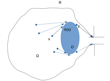
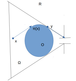
We consider different PDE modeling for crowd motion scenarios, or other sort of fluid flows, and we insert in the given domain $ R $ an obstacle $ O $. We then compute the shape derivatives of a cost functional, the average exit time, in order to be able to optimize the geometry of the obstacle $ O $ and so to minimize the average exit time of particles in the domain $ R $. This computation can be used to derive numerical simulations and understand whether the presence of an obstacle is or not profitable for the evacuation, or to optimize its shape and position, for instance when the presence of a structure (column, …) is already necessary in the building plan of a public space.
Citation: Boubacar Fall, Filippo Santambrogio, Diaraf Seck. Shape derivative for obstacles in crowd motion[J]. Mathematics in Engineering, 2022, 4(2): 1-16. doi: 10.3934/mine.2022012
We consider different PDE modeling for crowd motion scenarios, or other sort of fluid flows, and we insert in the given domain $ R $ an obstacle $ O $. We then compute the shape derivatives of a cost functional, the average exit time, in order to be able to optimize the geometry of the obstacle $ O $ and so to minimize the average exit time of particles in the domain $ R $. This computation can be used to derive numerical simulations and understand whether the presence of an obstacle is or not profitable for the evacuation, or to optimize its shape and position, for instance when the presence of a structure (column, …) is already necessary in the building plan of a public space.

| [1] |
D. Alexander, I. Kim, Y. Yao, Quasi-static evolution and congested crowd transport, Nonlinearity, 27 (2014), 1–36. doi: 10.1088/0951-7715/27/1/1

|
| [2] | L. Ambrosio, N. Gigli, G. Savaré, Gradient flows in metric spaces and in the spaces of probability measures, Birkhäuser: ETH Zurich, 2005. |
| [3] | D. Braess, Über ein Paradoxon aus der Verkehrsplanung, Unternehmensforschung, 12 (1969), 258–268. |
| [4] | M. C. Delfour, J. P. Zolésio, Shapes and Geometries, metrics, analysis, differential calculus, and optimization, 2 Eds., Philadelphia, USA: Society for Industrial and Applied Mathematics, 2011. |
| [5] |
S. Di Marino, A. Mészáros, Uniqueness issues for evolutive equations with density constraints, Math. Mod. Meth. Appl. Sci., 26 (2016), 1761–1783. doi: 10.1142/S0218202516500445
|
| [6] | T. Gasparotto, A. Collin, P. Boulet, G. Piante, A. Muller, Modélisation macroscopique de l'évacuation des personnes en situation d'incendie, In: proceedings of the 2016 conference of the French Thermic Society, Toulouse, 2018. |
| [7] | D. Helbing, A fluid dynamic model for the movement of pedestrians, Complex Syst., 6 (1992), 391–415. |
| [8] | A. Henrot, M. Pierre, Variation et optimisation de formes: Une analyse géométrique, Springer, 2005. |
| [9] | A. Henrot, M. Pierre, Shape variation and optimization A geometrical analysis, EMS, 2018. |
| [10] |
R. L. Hughes, A continuum theory for the flow of pedestrian, Transport. Res. B Meth., 36 (2002), 507–535. doi: 10.1016/S0191-2615(01)00015-7
|
| [11] |
R. Jordan, D. Kinderlehrer, F. Otto, The variational formulation of the Fokker-Planck equation, SIAM J. Math. Anal., 29 (1998), 1–17. doi: 10.1137/S0036141096303359
|
| [12] |
B. Maury, A. Roudneff-Chupin, F. Santambrogio, A macroscopic crowd motion model of gradient flow type, Math. Mod. Meth. Appl. Sci., 20 (2010), 1787–1821. doi: 10.1142/S0218202510004799
|
| [13] | B. Maury, A. Roudneff-Chupin, F. Santambrogio, J. Venel, Handling congestion in crowd motion modeling, Net. Het. Media, 6 (2011), 485–519. |
| [14] | B. Maury, J. Venel, Handling of contacts in crowd motion simulations, In: Traffic and granular flow '07, Berlin, Heidelberg: Springer, 2007,171–180. |
| [15] |
A. R. Mészáros, F. Santambrogio, Advection-diffusion equations with density constraints, Analysis PDE, 9 (2016), 615–644. doi: 10.2140/apde.2016.9.615
|
| [16] |
F. Otto, The geometry of dissipative evolution equations: The porous medium equation, Commun. Part. Diff. Eq., 26 (2001), 101–174. doi: 10.1081/PDE-100002243
|
| [17] | A. Roudneff-Chupon, Modélisation macroscopique de mouvements de foule, PhD thesis, Université Paris-Sud, 2011. |
| [18] | F. Santambrogio, Optimal transport for applied mathematicians, Basel: Birkhäuser, 2015. |
| [19] |
F. Santambrogio, $\{$Euclidean, metric, and Wasserstein$\}$ gradient flows: an overview, Bull. Math. Sci., 7 (2017), 87–154. doi: 10.1007/s13373-017-0101-1
|
| [20] |
F. Santambrogio, Crowd motion and population dynamics under density constraints, ESAIM Proceedings, 64 (2018), 137–157. doi: 10.1051/proc/201864137
|
| [21] | J. Sokolowski, J. P. Zolésio, Introduction to shape optimization. Shape sensivity analysis, Springer, 1992. |
| [22] |
E. Sandier, S. Serfaty, Gamma-convergence of gradient flows with applications to Ginzburg-Landau, Commun. Pure Appl. Math., 57 (2004), 1627–1672. doi: 10.1002/cpa.20005
|
| [23] | J. Venel, Modélisation mathématique et numérique de mouvements de foule, PhD thesis, Uni- versité Paris-Sud, 2008. |
| [24] |
D. Yanagisawa, A. Kimura, A. Tomoeda, R. Nishi, Y. Suma, K. Ohtsuka, et al., Introduction of frictional and turning function for pedestrian outflow with an obstacle, Phys. Rev. E, 80 (2009), 036110. doi: 10.1103/PhysRevE.80.036110
|
| [25] | C. Villani, Topics in optimal transportation, AMS, 2003. |
| [26] | M. T. Wolfram, personal communication, 2017. |
Figures(2)

Boubacar Fall, Filippo Santambrogio, Diaraf Seck. Shape derivative for obstacles in crowd motion[J]. Mathematics in Engineering, 2022, 4(2): 1-16. doi: 10.3934/mine.2022012


 DownLoad: