Improvement of saffron production using <em>Curtobacterium herbarum</em> as a bioinoculant under greenhouse conditions

Alexandra Díez-Méndez; Raul Rivas; Alexandra Díez-Méndez; Raul Rivas

doi:10.3934/microbiol.2017.3.354

AIMS Microbiology

2017, Volume 3, Issue 3: 354-364. doi: 10.3934/microbiol.2017.3.354

Previous Article Next Article

Research article Special Issues

Improvement of saffron production using Curtobacterium herbarum as a bioinoculant under greenhouse conditions

Alexandra Díez-Méndez ^1,2,
Raul Rivas ^{1,2,3
,
,}

1.
Department of Microbiology and Genetics, Edificio Departamental de Biología, Universidad de Salamanca, (USAL) Dres. de la Reina s/n, 37007, Salamanca, Spain
2.
Instituto Hispano Luso de Investigaciones Agrarias (CIALE), Salamanca, Spain
3.
Associated Unit USAL-CSIC (IRNASA), Salamanca, Spain

Received: 14 March 2017 Accepted: 16 May 2017 Published: 22 May 2017

Plant Growth Promoting Rhizobacteria (PGPR) are natural soil bacteria which establish a beneficial relationship with their host. This microbiota community exists in the rhizosphere and inside plant tissues and stimulates plant growth by a variety of direct or indirect mechanisms. These bacterial plant promoters are frequently present in different environments, and are associated with many plant species, both wild and agricultural. Saffron is the dried stigmas of Crocus sativus (L.) and is the most expensive spice in the world. Remarkably, saffron cultivation and collection is carried out by hand and does not involve the use of machines. Additionally, 150 flowers are needed to produce one gram of dried stigmas. Hence, a slight increase in the size of the saffron filaments per plant would result in a significant increase in the production of this spice. In this study, we report the improved production of saffron using Curtobacterium herbarum Cs10, isolated from Crocus seronitus subs clusii, as a bioinoculant. The bacterial strain was selected owing to its multifunctional ability to produce siderophores, solubilize phosphate and to produce plant growth hormones like IAA. Furthermore, the isolate was tested on saffron producing plants under greenhouse conditions. The results indicate that Curtobacterium herbarum Cs10 improves the number of flowers and significantly enhances the length of the saffron filaments and overall saffron production compared to the control treated plants.

Keywords:

Citation: Alexandra Díez-Méndez, Raul Rivas. Improvement of saffron production using Curtobacterium herbarum as a bioinoculant under greenhouse conditions[J]. AIMS Microbiology, 2017, 3(3): 354-364. doi: 10.3934/microbiol.2017.3.354

Related Papers:

[1]	Sathyanarayanan Gopalakrishnan, Swaminathan Venkatraman . Prediction of influential proteins and enzymes of certain diseases using a directed unimodular hypergraph. Mathematical Biosciences and Engineering, 2024, 21(1): 325-345. doi: 10.3934/mbe.2024015
[2]	Boyang Wang, Wenyu Zhang . MARnet: multi-scale adaptive residual neural network for chest X-ray images recognition of lung diseases. Mathematical Biosciences and Engineering, 2022, 19(1): 331-350. doi: 10.3934/mbe.2022017
[3]	Feng Wang, Xiaochen Feng, Ren Kong, Shan Chang . Generating new protein sequences by using dense network and attention mechanism. Mathematical Biosciences and Engineering, 2023, 20(2): 4178-4197. doi: 10.3934/mbe.2023195
[4]	Boyang Wang, Wenyu Zhang . ACRnet: Adaptive Cross-transfer Residual neural network for chest X-ray images discrimination of the cardiothoracic diseases. Mathematical Biosciences and Engineering, 2022, 19(7): 6841-6859. doi: 10.3934/mbe.2022322
[5]	Yongyin Han, Maolin Liu, Zhixiao Wang . Key protein identification by integrating protein complex information and multi-biological features. Mathematical Biosciences and Engineering, 2023, 20(10): 18191-18206. doi: 10.3934/mbe.2023808
[6]	Shun Li, Lu Yuan, Yuming Ma, Yihui Liu . WG-ICRN: Protein 8-state secondary structure prediction based on Wasserstein generative adversarial networks and residual networks with Inception modules. Mathematical Biosciences and Engineering, 2023, 20(5): 7721-7737. doi: 10.3934/mbe.2023333
[7]	Shuai Cao, Biao Song . Visual attentional-driven deep learning method for flower recognition. Mathematical Biosciences and Engineering, 2021, 18(3): 1981-1991. doi: 10.3934/mbe.2021103
[8]	Jinmiao Song, Shengwei Tian, Long Yu, Qimeng Yang, Qiguo Dai, Yuanxu Wang, Weidong Wu, Xiaodong Duan . RLF-LPI: An ensemble learning framework using sequence information for predicting lncRNA-protein interaction based on AE-ResLSTM and fuzzy decision. Mathematical Biosciences and Engineering, 2022, 19(5): 4749-4764. doi: 10.3934/mbe.2022222
[9]	Peter Hinow, Edward A. Rietman, Sara Ibrahim Omar, Jack A. Tuszyński . Algebraic and topological indices of molecular pathway networks in human cancers. Mathematical Biosciences and Engineering, 2015, 12(6): 1289-1302. doi: 10.3934/mbe.2015.12.1289
[10]	Babak Khorsand, Abdorreza Savadi, Javad Zahiri, Mahmoud Naghibzadeh . Alpha influenza virus infiltration prediction using virus-human protein-protein interaction network. Mathematical Biosciences and Engineering, 2020, 17(4): 3109-3129. doi: 10.3934/mbe.2020176

Abstract

1. Introduction

The proteins contained in the biological membrane are called membrane proteins, which play a lead role in maintaining many life activities, including but not limited to cell proliferation and differentiation, energy transformation, signal transduction and material transportation. As we know, a membrane protein's functions are significantly associated with its type, so it is important to identify the types of membrane proteins ^[1]. Membrane proteins can be grouped into eight types ^[2]: Single-span type 1, single-span type 2, single-span type 3, single-span type 4, multi-span, lipid-anchor, glycosylphosphatidylinositol (GPI)-anchor and peripheral.

There exists many different computational methods that can be used for identifying the types of proteins. Chou and Elrod ^[3] used the covariant discriminant algorithm (CDA) according to amino acid composition (AAC) to predict membrane protein types. To address the challenge posed by the large number of possible patterns in protein sequences, Chou ^[4] introduced a pseudo-amino acid composition (PAAC). This composition combines a set of discrete sequence correlation factors with the 20 components of the traditional amino acid composition. Wang et al. ^[5] utilized the pseudo amino acid composition to incorporate sequence-order effects and introduced spectral analysis for representing the statistical sample of a protein. The weighted support vector machine (SVM) algorithm was applied. Liu et al. ^[6] introduced the low-frequency Fourier spectrum analysis based on the concept of PAAC, which effectively incorporates sequence patterns into discrete components and enables existing prediction algorithms to be applied directly to protein samples. Chou and Shen ^[7] developed a two-layer predictor for classifying proteins as membrane or non-membrane. If a protein is classified as membrane, the process continues with a second-layer prediction engine to determine its specific type from eight categories. The predictor stands out for its incorporation of evolutionary information through pseudo position-specific score matrix (Pse-PSSM) vectors and its ensemble classifier consisting of multiple optimized evidence-theoretic K-nearest neighbor (OET-KNN) classifiers. Rezaei et al. ^[8] classified membrane proteins by applying wavelet analysis to their sequences and extracting informative features. These features were normalized and used as input for a cascaded model, which aimed to mitigate bias caused by differences in membrane protein class sizes in the dataset. Wang et al. ^[9] utilized the dipeptide composition (DC) method to represent proteins as high-dimensional feature vectors. They introduced the neighborhood preserving embedding (NPE) algorithm for linear dimensionality reduction and to extract essential features from the high-dimensional DC space. The reduced low-dimensional features were then employed with the K-nearest neighbor (K-NN) classifier to accurately classify membrane protein types. Hayat and Khan ^[10] integrated composite protein sequence features (CPSR) with the PAAC to classify membrane protein. They further proposed using split amino acid composition (SAAC) and ensemble classification ^[11] and still further fused position specific scoring matrix (PSSM) and SAAC ^[12] to classify membrane protein. Chen and Li ^[13] introduced a novel computational classifier designed for the prediction of membrane protein types using protein sequences. The classifier was constructed based on a collection of one-versus-one SVMs and incorporated various sequence attributes. Han et al. ^[14] integrated amino acid classifications and physicochemical properties in PAAC and used a two-stage multiclass SVM to classify membrane protein. Wan et al. ^[15] retrieved the associated gene ontology (GO) information of a query membrane protein by searching a compact GO-term database with its homologous accession number. Subsequently, they employed a multi-label elastic net (EN) classifier to classify the membrane protein based on this information. Lu et al. ^[16] used a dynamic deep network architecture that was based on lifelong learning for the classification of membrane protein. Wang et al. ^[17] introduced a new support bio-sequence machine, which used SVM for protein classification.

In conclusion, most of the above models used different computational methods to represent membrane proteins and then used classification algorithms to identify membrane protein types. Most of the models mentioned above have varied types of feature input formats, which are shown in Table 1.

Table 1. Varied types of feature input formats of different methods.

Methods	Input form
MemType-2L ^[7]	Pseudo-PSSM (PsePSSM)
predMPT ^[13]	Pseudo amino acid composition
CDA ^[3]	Amino acid composition
CDA and PseAA ^[4]	Pseudo amino acid composition
Fourier spectrum ^[6]	Pseudo amino acid composition
Weighted SVM ^[5]	Pseudo amino acid composition
Wavelet and cascade neural network ^[8]	Hydropathy signal
NPE ^[9]	Dimension-reduced vector(50-D) by NPE
CPSR ^[10]	Pseudo amino acid composition
Two-stage SVM ^[14]	Pseudo amino acid composition

| Show Table

DownLoad: CSV

However, it is noted that more than two proteins are linked by non-covalent interactions ^[18,19] in real practice, and the representation of proteins is multi-modal. Traditional computational methods for identifying membrane protein types tend to ignore those two issues, which leads to information loss since the high-order correlation among membrane proteins and the scenarios of multi-modal representations of membrane proteins are ignored.

To tackle those problems, in this paper we use a deep residual hypergraph neural network (DRHGNN) ^[20] to further learn about the representations of membrane proteins and to eventually achieve accurate identification of membrane proteins' types.

First, each membrane protein is represented by the extracted features. Here, five feature extraction methods are employed based on the PSSM of membrane protein sequence ^[2], including average blocks (AvBlock), discrete cosine transform (DCT), discrete wavelet transform (DWT), histogram of oriented gradient (HOG) and PsePSSM. Five types of features are extracted accordingly. Second, each feature type generates a hypergraph G represented by an incidence matrix H modeling complex high-order correlation. Five types of features and corresponding incidence matrix H are concatenated, respectively, which overcomes the scenarios of multi-modal representations of membrane proteins. Lastly, concatenated features and fused incidence matrix are input into a DRHGNN to classify the various types of membrane proteins. To assess the performance of DRHGNN, we perform tests on membrane proteins' four distinct datasets. In the task of membrane proteins classification, the model achieves better performance.

2. Materials and methods

In order to extract features of membrane proteins, we employ AvBlock, DCT, DWT, HOG and PsePSSM ^[2] to achieve feature extraction based on membrane protein sequence's PSSM. Each type of PSSM-based feature is used to generate a hypergraph that can be represented by an incidence matrix H, then five types of features and their corresponding H are concatenated, respectively, and both are fed into a DRHGNN ^[20,21,22] to identify the types of membrane proteins. Figure 1 depicts the schematic diagram.

Figure 1. The schematic diagram of our proposed method.

DownLoad: Full-Size Img PowerPoint

2.1. Data set

We judge the performance of DRHGNN on the classification of membrane proteins based on four datasets, namely, Dataset 1, Dataset 2, Dataset 3 and Dataset 4.

Dataset 1 is directly sourced from Chou's work ^[7], where protein sequences are sourced from the Swiss-Prot ^[23] database. Chou and Shen ^[7] employed a percentage distribution method to randomly assign the protein sequences into both the training set and the testing set. This was done to ensure a balanced number of sequences between the two sets. Dataset 1 consists of 7582 membrane proteins from eight types and the same training/testing split as ^[7], where 3,249 membrane proteins are employed for training, with the remaining 4,333 employed for testing.

Dataset 2 was created by removing redundant and highly similar sequences from Dataset 1. This resulted in a curated dataset with reduced homology, specifically ensuring that no pair of proteins shared a sequence identity greater than 40%. The training set of Dataset 2 was obtained by removing redundant sequences from Dataset 1's training set. Similarly, the testing set of Dataset 2 was prepared by eliminating redundant sequences and those with high sequence identity to the training set. Dataset 2 consists of 4594 membrane proteins from eight types and the same training/testing split as ^[13], where 2288 membrane proteins are employed for training, with the remaining 2306 membrane proteins employed for testing.

To update and expand the datasets, Chen and Li ^[13] created Dataset 3 through the following steps. Initially, membrane protein sequences were obtained from the Swiss-Prot ^[23] database using the "protein subcellular localization" annotation. Stringent exclusion criteria was applied to ensure dataset quality: 1) Exclusion of fragmented proteins or those shorter than 50 amino acid residues; 2) removal of proteins with non-experimental qualifiers or multiple topologies in their annotations; 3) elimination of homologous sequences with a sequence identity greater than 40% using clustering database at high identity with tolerance (CD-hit) ^[24]. Subsequently, the sequences were categorized into their respective membrane protein types based on topology annotations. To generate the training and testing sets, a random assignment was performed employing the above-mentioned percentage distribution method. Consequently, Dataset 3 was created, providing an updated and expanded dataset of membrane protein sequences characterized by enhanced quality and classification. Dataset 3 consists of 6677 membrane proteins from eight types and the same training/testing split as ^[13], where 3,073 membrane proteins are employed for training and 3604 for testing.

Dataset 4 is directly sourced from Chou's work ^[3], where protein sequences are sourced from the Swiss-Prot ^[23] database. The training and testing sets were obtained after protein sequences were screened with three procedures. Dataset 4 consists of 4684 membrane proteins from five types and the same training/testing split as ^[3], where 2059 membrane proteins are used for training and 2625 membrane proteins are employed for testing. Table 2 outlines the details of the datasets.

Table 2. The scale of training and testing samples in four different membrane proteins' datasets.

Specific types	Dataset 1		Dataset 2		Dataset 3		Dataset 4
Specific types	Train	Test	Train	Test	Train	Test	Train	Test
Single-span type 1	610	444	388	223	561	245	435	478
Single-span type 2	312	78	218	39	316	7	152	180
Single-span type 3	24	6	19	6	32	9	–	–
Single-span type 4	44	12	35	10	65	17	–	–
Multi-span type 5	1316	3265	936	1673	1119	2478	1311	1867
Lipid-anchor type 6	151	38	98	26	142	36	51	14
GPI-anchor type 7	182	46	122	24	164	41	110	86
Peripheral type 8	610	444	472	305	674	699	–	–
Overall	3249	4333	2288	2306	3073	3604	2059	2625

| Show Table

DownLoad: CSV

We use the same membrane protein features as ^[2], which are extracted with five methods based on the PSSM of membrane proteins.

2.2. PSSM

The PSSM is a widely used tool in the field of bioinformatics for capturing evolutionary information encoded within membrane protein sequences. It is generated through multiple sequence alignment and database searching methods, such as position-specific iterated BLAST (PSIBLAST) program ^[25], to identify conserved residues and their positional probabilities.

The evolutionary information obtained from the PSSM is preserved within a matrix of size R $\times$ 20 (R rows and 20 columns), presented as follows:

$\begin{equation} PSSM = \left(\begin{array}{ccccc} p_{1,1} & \cdots & p_{1, j} & \cdots & p_{1,20} \\ \vdots & \ddots & \vdots & \ddots & \vdots \\ p_{i, 1} & \cdots & p_{i, j} & \cdots & p_{i, 20} \\ \vdots & \ddots & \vdots & \ddots & \vdots \\ p_{R, 1} & \cdots & p_{R, j} & \cdots & p_{R, 20} \end{array}\right). \end{equation}$

(2.1)

The numbers 1–20 denote one of the 20 different amino acids. R denotes the length of the membrane protein sequence.The element $p_{i, j}$ is calculated as follows:

$\begin{equation} p_{i, j} = \sum\limits_{k = 1}^{20} \omega(i, k) \times D(k, j) ; i = 1, \ldots, L, j = 1, \ldots, 20. \end{equation}$

(2.2)

$\omega(i, k)$ represents the frequency of the k-th amino acid type at position i, and D(k, j) denotes the value derived from Dayhoff's mutation matrix (substitution matrix) for the k-th and j-th amino acid types. The utilization of these variables in the equation aims to incorporate amino acid frequency information and substitution probabilities.

2.3. AvBlock

AvBlock refers to a statistical measure employed in professional scientific research to analyze data sequences. Nowadays, AvBlock is a widely adopted approach for constructing matrix descriptors to represent protein sequences ^[26]. AvBlock is calculated by dividing the total length of a sequence by the average length of its individual consecutive blocks. Here, the PSSM matrix is partitioned into 20 blocks along the rows. Subsequently, each block is transformed into a feature vector of dimensionality 20 for the PSSM matrix.

2.4. DCT

The DCT ^[27] is a mathematical transform widely used in signal and image processing. Here, we employ a two-dimensional DCT (2D-DCT) for compressing the PSSM of proteins. The mathematical definition for the 2D-DCT is

$\begin{equation} \begin{array}{l} F_{P S S M-D C T} = \alpha_{i} \alpha_{j} \sum _{m = 0}^{M-1} \sum _{n = 0}^{N-1} P S S M(m, n) \cos \frac{\pi(2 m+1) i}{2 M} \cos \frac{\pi(2 n+1) j}{2 N} \\ \end{array} \end{equation}$

(2.3)

$\begin{equation} \alpha_{i} = \left\{\begin{array}{ll} \sqrt{1 / M}, & i = 0 \\ \sqrt{2 / M}, & 1 \leq i \leq M-1 \end{array}\right. \end{equation}$

(2.4)

$\begin{equation} \alpha_{j} = \left\{\begin{array}{ll} \sqrt{1 / N}, & j = 0 \\ \sqrt{2 / N}, & 1 \leq j \leq N-1, \end{array}\right. \end{equation}$

(2.5)

where 0 $< i < M$ and $0 < j < N$ .

2.5. DWT

The DWT has been utilized to extract informative features from protein amino acid sequences, as initially introduced by Nanni et al. ^[28]. Here, we applied a 4-level DWT to preprocess the PSSM matrix. At each level we compute both the approximate and detailed coefficients for each column. We extract essential statistical features such as maximum, minimum, mean and standard deviation from both the approximate and detailed coefficients. Additionally, we capture the first five discrete cosine coefficients exclusively from the approximate coefficients. Therefore, for each of the 20 column dimensions, a total of $4+4+5$ features are obtained at each level.

2.6. HOG

The HOG is a feature descriptor used in computer vision and image processing for object detection and recognition. Here, we propose a method to reduce redundancy in protein data using the HOG algorithm. We consider the PSSM as an image-like matrix representation. First, we compute the horizontal and vertical gradients of the PSSM to obtain the gradient magnitude and direction matrices. These matrices are then partitioned into 25 sub-matrices that incorporate both the gradient magnitude and direction information. Subsequently, we generate 10 distinct histogram channels for each sub-matrix based on its gradient direction. This approach effectively reduces redundancy by providing a compact representation of the protein data while preserving important spatial information.

2.7. PsePSSM

The PsePSSM is a commonly utilized matrix descriptor in protein research ^[7]. It is specifically designed to preserve the essential information contained in the PSSM by considering the incorporation of PAAC. The PsePSSM descriptor is formulated as follows:

$\begin{equation} F_{P s e P S S M} = \left\{\begin{array}{l} \frac{1}{N} \sum _{i = 1}^{N} p_{i, j}^{\prime} ; j = 1, \ldots, 20 \\ \frac{1}{N-l a g} \sum _{i = 1}^{N-l a g}\left(p_{i, j}^{\prime}-p_{i+l a g, j}^{\prime}\right)^{2} ; j = 1, \ldots, 20, \text { lag } = 1, \ldots, 30, \end{array}\right. \end{equation}$

(2.6)

where lag refers to the distance between a residue and its neighboring residues. The formula of $p_{i, j}^{\prime}$ is

$\begin{equation} p_{i, j}^{\prime} = \frac{p_{i, j}-\frac{1}{20} \sum _{m = 1}^{20} p_{i, m}}{\sqrt{\frac{1}{20} \sum _{n = 1}^{20}\left(p_{i, n}-\frac{1}{20} \sum _{m = 1}^{20} p_{i, m}\right)^{2}},} \end{equation}$

(2.7)

where $p_{i, j}^{\prime}$ refers to the normalized version of $p_{i, j}$ .

2.8. DRHGNN

2.8.1. Hypergraph learning statement

In a basic graph, the samples are depicted as vertexes, and two connected vertexes are joined by an edge ^[29,30]. However, the data structure in practical applications may go beyond pair connections and may even be multi-modal. Accordingly, the hypergraph was proposed. Unlike the simple graph, a hypergraph comprises a vertex set and one or more hyperedge set(s) composed of two or more vertexes, as shown in . A hypergraph is represented by G = (V, E, W), where V represents a vertex set, and E represents a hyperedge set. W, a diagonal matrix of edge weights, assigns weights to each hyperedge. The incidence matrix H, where H is the $|V| \times|E|$ incidence matrix with entries defined as

$\begin{equation} h(v, e) = \left\{\begin{array}{l} 1 , \text { if } v \in \mathrm{e} \\ 0 , \text { if } v\notin \mathrm{e,} \end{array}\right. \end{equation}$

(2.8)

Figure 2. The comparison between graph and hypergraph.

DownLoad: Full-Size Img PowerPoint

is used to denote the hypergraph.

Here, we could take the membrane protein classification task on the hypergraph because more than two proteins are linked by non-covalent interactions ^[18,19]. $X = \left[\mathrm{x}_1, \ldots, \mathrm{x}_{\mathrm{N}}\right]^{\mathrm{T}}$ can represent the features of N membrane proteins data. The hyperedge is constructed using the Euclidean distance, which calculates the distance expressed with $\mathrm{d}\left(\mathrm{x}_{\mathrm{i}}, \mathrm{x}_{\mathrm{j}}\right)$ between two features. In the hyperedge construction, each vertex represents a membrane protein, and then one central vertex and its K neighbors represent each hyperedge. As a result, N hyperedges containing K+1 vertexes are generated. Here, more specifically, each time we select one vertex in the dataset as the centroid, we use K nearest neighbors in the selected feature space to generate one hyperedge, which includes the centroid itself, as illustrated in . Thus, a hypergraph with N hyperedges is constructed with a single-modal representation of membrane proteins. The hypergraph is denoted by an incidence matrix $\mathrm{H} \in \mathrm{R}^{\mathrm{NxN}}$ , with Nx(K+1) nonzero entries denoting $v \in e$ while the others equal zero.

Figure 3. The schematic diagram of hyperedge generation and hypergraph generation.

DownLoad: Full-Size Img PowerPoint

In the case of multi-modal representations of membrane proteins, each incidence matrix $H_i$ is constructed according to each modality membrane representation. After all the incidence matrix $H_i$ have been generated, these $H_i$ can be concatenated to generate the incidence matrix $H$ of a multi-modality hypergraph. Thus, a hypergraph is constructed with multi-modal representations of membrane proteins shown in Figure 3, so it is noted that the flexibility of hypergraph generation has great expansibility toward multi-modal features.

2.8.2. Hypergraph convolution

Feng et al. ^[31] first proposed the HGNN. They built a hyperedge convolution layer whose formulation is

$\begin{equation} \mathrm{X}^{(1+1)} = \sigma\left(\mathrm{D}_{\mathrm{v}}^{-1 / 2} \mathrm{HWD}_{\mathrm{e}}^{-1} \mathrm{H}^{\mathrm{T}} \mathrm{D}_{\mathrm{v}}^{-1 / 2} \mathrm{X}^{(1)} \Theta^{(1)}\right), \end{equation}$

(2.9)

where $X^{(l)} \in R^{N x C}$ represents the hypergraph's signal at the lth layer with N nodes and C dimensional features, W is regarded as the weight of all hyperedges and $W = \operatorname{diag}\left(w_{1}, \ldots, w_{N}\right). \Theta^{(l)} \in R^{C_{1} x C_{2}}$ represents the parameter that is learned during the training process at the lth layer. $\sigma$ represents the nonlinear activation function. $D_{v}$ is the vertex degrees' diagonal matrix, while $D_{e}$ is the edge degrees' diagonal matrix ^[30].

We define hypergraph Laplacian $\widetilde{H} = D_{v}^{-1 / 2} H W D_{e}^{-1} H^{T} D_{v}^{-1 / 2}$ , then a hyperedge convolution layer is formulated as $X^{(l+1)} = \sigma\left(\widetilde{H} X^{(l)} \Theta^{(l)}\right)$ .

A hyperedge convolution layer achieves node-edge-node transform, which can refine a better representation of nodes and extract the high-order correlation from a hypergraph more efficiently.

2.8.3. Residual hypergraph convolution

Feng et al. ^[31] used two hyperedge convolution layers and then used the softmax function to obtain predicted labels. However, the performance of HGNN drops as the number of layers increases because of the over-smoothing issue.

To resolve the issue of over-smoothing, Huang et al. ^[20] and Chen et al. ^[22] used two simple and effective techniques, Initial residual and identity mapping, based on their shallow model. Inspired by their method, we upgrade the HGNN by introducing initial residual and identity mapping to prevent over-smoothing and enjoy accuracy increase from increased depth.

● Initial residual

Chen et al. ^[22] constructed a connection to the initial representation $X^{(0)}$ to relieve the over-smoothing problem. The initial residual connection guarantees that each node's final representation retains at least a proportion of the input feature regardless of how many layers we stack.

Gasteiger et al. ^[32] proposed approximate personalized propagation of neural predictions (APPNP), which employed a linear combination between different layers to the initial residual connection and gathered information from multi-hop neighbors instead of expanding the number of neural network layers by separating feature transformation and propagation. Formally, APPNP's model is defined as

$\begin{equation} X^{(l+1)} = \sigma\left(\left(\left(1-\alpha_{l}\right) \widetilde{H} X^{(l)}+\alpha_{l} X^{(0)}\right) \Theta^{(l)}\right). \end{equation}$

(2.10)

In practice, we can set $\alpha_{l} = 0.1 \quad or \quad 0.2$ .

● Identity mapping

However, APPNP remains a shallow model; thus, the initial residual alone cannot extend HGNN to a deep model. To resolve this issue, Chen et al. ^[22] added an identity matrix $I_{N}$ to the weight matrix $\Theta ^{(l)}$ according to the idea in ResNet of identity mapping, which ensures the DRHGNN model performs at least as well as its shallow version does.

Finally, a residual enhanced hyperedge convolution layer is formulated as

$\begin{align} X^{(l+1)} & = \sigma\left(\left(\left(1-\alpha_{l}\right) \widetilde{H} X^{(l)}+\alpha_{l} X^{(0)}\right) \right. \left. \cdot \left(\left(1-\beta_{l}\right) I_{n}+\beta_{l} \Theta^{(l)}\right)\right). \end{align}$

(2.11)

In practice, we set $\beta_{l} = \frac{\lambda }{l}$ , where $\lambda$ is a hyperparameter.

2.8.4. DRHGNN analysis

Figure 4 illustrates the detail of the DRHGNN. Those multi-types of node features and corresponding incidence matrix H modeling complex high-order correlation are concatenated, respectively, which overcomes the scenarios of multi-modal representations of membrane proteins. Then, concatenated features and incidence matrix are fed into DRHGNN to get nodes output labels and eventually achieve classification task. As detailed in the section mentioned above, we can build a residual enhanced hypergraph convolution layer, then we naively stack multiple residual hypergraph convolution blocks to tackle the problem of over-smoothing in HGNN and enjoy an accuracy increase. Additional linear transforms are incorporated into the model's first and last layer, and the residual hypergraph convolutions are utilized for information propagation. The deep embeddings are finally used for classification tasks.

Figure 4. The DRHGNN framework. FC represents a fully connected layer.

DownLoad: Full-Size Img PowerPoint

3. Results

3.1. Hyperparameter settings based on experience

The DRHGNN has numerous hyperparameters. Instead of comparing all the possible hyperparameters, which usually takes several days, we used empirically based hyperparameters, which are shown in Table 3.

Table 3. Hyperparameters used in this study.

Hyperparameters	Setting
Epoch	2000
Learning rate	0.001
Hidden layer	128
Dropout rate	0.5
Activation function	ReLU+Softmax
Optimizer	Adam
Loss function	Cross-entropy loss function
$\alpha$	0.1
$\lambda$	2.5

| Show Table

DownLoad: CSV

We implemented our model with Pytorch ^[33].

The baseline results were replicated by their release codes, with hyperparameters adhering to the respective papers.

3.2. Metrics

We conducted accuracy calculations for predicting every type of membrane protein. We used accuracy (ACC), which measures the ratio of correctly predicted proteins to the total number of proteins in a specified dataset, to assess the performance of our model. The specific formula is

$\begin{equation} ACC = \frac{n}{N}, \end{equation}$

(3.1)

where n stands for the number of proteins that are correctly predicted in a specified dataset, and N stands for the total number of proteins present in the dataset.

In order to further evaluate the performance of models, we also incorporated F1-score and Mathew's correlation coefficient (MCC) as evaluation metrics.

The F1-score is a useful metric for addressing the issue of imbalanced datasets, which is composed of precision and recall. Precision refers to the ratio of the number of correctly predicted samples to the total number of samples predicted as positive, while recall refers to the ratio of the number of correctly predicted samples to the total number of actual positive samples. The best value of F1-score is 1, while the worst value is 0. Their specific formulas are

$\begin{equation} \text { F1-score } = 2 \times \frac{\text { Precision } \times \text { Recall }}{(\text { Precision }+ \text { Recall })} \end{equation}$

(3.2)

$\begin{equation} \text { Precision } = \frac{T P}{T P+F P} \end{equation}$

(3.3)

$\begin{equation} \text { Recall } = \frac{T P}{T P+F N}, \end{equation}$

(3.4)

where TP, TN, FP and FN are true positive, true negative, false positive and false negative, respectively.

In order to comprehensively evaluate the F1-scores of multiple classes, we employed the macro average of F1-score, which aggregates the F1-score for different classes by taking their average with equal weights assigned to all classes.

MCC is widely acknowledged as a superior performance metric for the classification of imbalanced data. It is defined within the range of $[-1, 1]$ , where a value of 1 indicates that the classifier accurately predicts all positive instances and negative instances, while a value of $-1$ signifies that the classifier incorrectly predicts all instances. The specific formula is

$\begin{equation} M C C(i) = \frac{T P \times T N-F P \times F N}{\sqrt{[T P+F P][T P+F N][T N+F P][T N+F N]}}. \end{equation}$

(3.5)

The overall MCC for all categories is computed by averaging the MCC values of individual categories.

3.3. The selection of K value when constructing the hypergraph

The selection of K neighbors plays a vital role in the construction process of the hyperedge, as it has a significant impact on the model's performance. The selection of K value is performed by training the model with different K values and evaluating its performance. The optimal K value is determined based on the performance metric obtained from the validation set. We performed K value experiments on four datasets using DRHGNN. The performance metric is macro average of the F1-score. As observed from , each dataset achieves the best experimental result at different K values, specifically $K = 8$ , 10, 12 and 2 respectively. Therefore, when conducting experiments on the four datasets, we selected K values in sequence as 8, 10, 12 and 2.

Table 4. The performance of DRHGNN with different K values on four datasets. The best result for each dataset is bolded.

Datasets	Metric	K
Datasets	Metric	2	4	6	8	10	12	14
Dataset 1	F1-score	0.68282	0.74181	0.73623	0.75769	0.75697	0.75656	0.74846
Dataset 2	F1-score	0.65046	0.65052	0.64668	0.67813	0.68646	0.68438	0.67955
Dataset 3	F1-score	0.57224	0.56307	0.59114	0.59234	0.58799	0.59317	0.59105
Dataset 4	F1-score	0.95651	0.94911	0.94645	0.95541	0.94468	0.94590	0.94242

| Show Table

DownLoad: CSV

3.4. Performance comparison of DRHGNN and HGNN with different layers

The performance of DRHGNN against HGNN with different layers on four datasets is reported in Table 5. Columns 4–9 show the ACC, macro average of the F1-score between DRHGNN and HGNN with different layers on four datasets. For better comparison, we presented the results in Figure 5. By analyzing Table 5 and Figure 5, we can observe two points: 1) DRHGNN achieves much better performance than HGNN on four datasets with accuracy gains of 3.738, 3.903, 4.106, 1.028%, respectively, and with a macro average of F1-score gains of 15.306, 11.843, 13.887, 3.591%, respectively, with their optimal layer. 2) The residual enhanced model (DRHGNN) has stable performance, while the performance of HGNN deteriorates as the number of layers increases. The potential reason for HGNN's performance degradation with increasing layer depth is that the model may suffer from an over-smoothing issue. The performance of DRHGNN persistently improves and achieves the best accuracy on four datasets at layer 4, 8, 4 and 8, respectively, and the best macro average of the F1-score on four datasets at layer 4, 8, 4 and 16, respectively.

Table 5. Comparison of the ACC, macro average of F1-score between DRHGNN and HGNN with different depths on four datasets. The best result of methods for each dataset is bolded.

Datasets	Methods	Metrics	Layers
Datasets	Methods	Metrics	2	4	8	16	32	64
Dataset 1	HGNN	ACC	0.90492	0.90122	0.88114	0.70688	0.75352	0.75352
	HGNN	F1-score	0.60463	0.46066	0.32800	0.27766	0.12858	0.11633
	DRHGNN	ACC	0.92799	0.94230	0.93492	0.93561	0.93330	0.93215
	DRHGNN	F1-score	0.68801	0.75769	0.73092	0.72435	0.75289	0.70492
Dataset 2	HGNN	ACC	0.86904	0.84996	0.80833	0.81049	0.72550	0.72550
	HGNN	F1-score	0.55921	0.42989	0.28404	0.28703	0.12723	0.11472
	DRHGNN	ACC	0.89072	0.89809	0.90807	0.89592	0.89245	0.89549
	DRHGNN	F1-score	0.66307	0.67684	0.67764	0.66848	0.65073	0.64934
Dataset 3	HGNN	ACC	0.85322	0.85294	0.81104	0.80549	0.68757	0.68785
	HGNN	F1-score	0.45430	0.37403	0.27717	0.26733	0.12236	0.11141
	DRHGNN	ACC	0.88957	0.89428	0.89179	0.88929	0.88873	0.88652
	DRHGNN	F1-score	0.59160	0.59317	0.57857	0.57942	0.57635	0.56952
Dataset 4	HGNN	ACC	0.96343	0.97562	0.96762	0.93486	0.71124	0.71124
	HGNN	F1-score	0.89026	0.93080	0.90231	0.75977	0.16625	0.16625
	DRHGNN	ACC	0.98590	0.98400	0.98590	0.98514	0.98133	0.98019
	DRHGNN	F1-score	0.95951	0.95651	0.96116	0.96671	0.95890	0.95858

| Show Table

DownLoad: CSV

Figure 5. The performance comparison of DRHGNN and HGNN with different layers on membrane protein classification task. (a) The performance comparison of DRHGNN and HGNN on Dataset 1; (b) The performance comparison of DRHGNN and HGNN on Dataset 2; (c) The performance comparison of DRHGNN and HGNN on Dataset 3; (d) The performance comparison of DRHGNN and HGNN on Dataset 4.

DownLoad: Full-Size Img PowerPoint

3.5. Performance comparison with multiple recently developed advanced methods

The summaries of classification accuracy results of DRHGNN with multiple recently developed advanced methods are shown in Tables 6–Table 9. Tables 6–Table 8 present a comparison of the accuracy of each type of membrane protein and the overall accuracy across all membrane proteins for Dataset 1, Dataset 2, and Dataset 3 using different methods. As Tables 6–Table 8 show, the accuracy of each type of membrane protein obtained using our method is generally higher than those achieved by other methods, and the overall accuracy is also superior to that of other methods. More specifically, compared with the MemType-2L ^[7] and hypergraph neural network ^[34] on Dataset 1, DRHGNN achieves overall accuracy gains of 2.63 and 3.738%, respectively. Compared with the MemType-2L ^[7] and hypergraph neural network ^[34] on Dataset 2, DRHGNN achieves overall accuracy gains of 5.507 and 3.903%, respectively. Compared with the MemType-2L ^[7] and hypergraph neural network ^[34] on Dataset 3, DRHGNN achieves overall accuracy gains of 11.128 and 4.106%, respectively. Furthermore, within these three datasets, the fifth type of membrane protein exhibits the highest accuracy compared to other types. This can potentially be attributed to the significantly larger number of samples available for the fifth type of membrane protein in these datasets. Table 9 presents a comparison of the overall accuracy between our proposed method and other methods on Dataset 4. As Table 9 shows, our method achieved the best performance among all the compared methods. More specifically, compared with CPSR ^[10] and two-stage SVM ^[14] on Dataset 4, DRHGNN achieves overall accuracy gains of 3.314 and 1.814%, respectively. Those results demonstrate the superior performance of DRHGNN on the membrane protein classification task. The detailed performance of DRHGNN on four datasets is shown in Table 10.

Table 6. Comparison of the ACC between DRHGNN and multiple recent state of the art methods on Dataset 1. The best result among methods is bolded.

Membrane protein types	Metric	MemType-2L ^[7]	Hypergraph neural network ^[34]	DRHGNN
Single-span type 1	ACC	0.86900	0.90090	0.93468
Single-span type 2	ACC	0.70500	0.34615	0.80769
Single-span type 3	ACC	0.33333	0.16667	0.33333
Single-span type 4	ACC	0.66667	0.33333	0.66667
Multi-span	ACC	0.95000	0.93813	0.96478
Lipid-anchor	ACC	0.42100	0.26316	0.55263
GPI-anchor	ACC	0.76100	0.63043	0.84783
Peripheral	ACC	0.82200	0.87162	0.86712
Overall	ACC	0.91600	0.90492	0.94230

| Show Table

DownLoad: CSV

Table 7. Comparison of the ACC between DRHGNN and multiple recent state of the art methods on Dataset 2. The best result among methods is bolded.

Membrane protein types	Metric	MemType-2L ^[7]	Hypergraph neural network ^[34]	DRHGNN
Single-span type 1	ACC	0.76700	0.77130	0.85650
Single-span type 2	ACC	0.66700	0.23077	0.64103
Single-span type 3	ACC	0.33333	0.16667,	0.16667
Single-span type 4	ACC	0.70000	0.40000	0.60000
Multi-span	ACC	0.91400	0.93843	0.94979
Lipid-anchor	ACC	0.23100	0.23077	0.26923
GPI-anchor	ACC	0.70800	0.58333	0.75000
Peripheral	ACC	0.68200	0.74754	0.84262
Overall	ACC	0.85300	0.86904	0.90807

| Show Table

DownLoad: CSV

Table 8. Comparison of the ACC between DRHGNN and multiple recent state of the art methods on Dataset 3. The best result among methods is bolded.

Membrane protein types	Metric	MemType-2L ^[7]	Hypergraph neural network ^[34]	DRHGNN
Single-span type 1	ACC	0.69000	0.60816	0.77959
Single-span type 2	ACC	0.58200	0.16456	0.40506
Single-span type 3	ACC	0.55600	0.11111	0.11111
Single-span type 4	ACC	0.52900	0.17647	0.29412
Multi-span	ACC	0.90700	0.93826	0.95642
Lipid-anchor	ACC	0.33333	0.08333	0.36111
GPI-anchor	ACC	0.65900	0.29268	0.73171
Peripheral	ACC	0.43900	0.81402	0.83119
Overall	ACC	0.78300	0.85322	0.89428

| Show Table

DownLoad: CSV

Table 9. Comparison of the ACC between DRHGNN and multiple recently developed advanced methods on Dataset 4. The best result among methods is bolded.

Methods	Input form	ACC
CDA ^[3]	Amino acid composition	0.79400
CDA and PseAA ^[4]	Pseudo amino acid composition	0.87500
Fourier spectrum ^[6]	Pseudo amino acid composition	0.87000
Weighted SVM ^[5]	Pseudo amino acid composition	0.90300
Wavelet and cascade neural network ^[8]	Hydropathy signal	0.91400
NPE ^[9]	Dimension-reduced vector(50-D) by NPE	0.90100
CPSR ^[10]	Pseudo amino acid composition	0.95200
Two-stage SVM ^[14]	Pseudo amino acid composition	0.96700
DRHGNN	PSSM-DCT+	0.98514
	PSSM-AvBlock+
	PSSM-DWT+
	PSSM-HOG+
	PsePSSM

| Show Table

DownLoad: CSV

Table 10. The detailed performance of DRHGNN on four datasets.

Membrane protein types	Metrics	Dataset 1	Dataset 2	Dataset 3	Dataset 4
Single-span type 1	ACC	0.93468	0.85650	0.77959	0.98536
	F1-score	0.92325	0.82773	0.80160	0.98312
	MCC	0.91445	0.84770	0.78271	0.98590
Single-span type 2	ACC	0.80769	0.64103	0.40506	0.98889
	F1-score	0.74556	0.63636	0.44330	0.93931
	MCC	0.74282	0.63485	0.42195	0.93091
Single-span type 3	ACC	0.33333	0.16667	0.11111	–
	F1-score	0.44444	0.36364	0.15385	–
	MCC	0.47091	0.23432	0.16530	–
Single-span type 4	ACC	0.66667	0.60000	0.29412	–
	F1-score	0.76190	0.75000	0.41667	–
	MCC	0.76927	0.77392	0.36325	–
Multi-span	ACC	0.96478	0.94979	0.95642	0.98500
	F1-score	0.97448	0.95333	0.95528	0.98952
	MCC	0.90025	0.84768	0.86025	0.96609
Lipid-anchor	ACC	0.55263	0.26923	0.36111	1.00000
	F1-score	0.58333	0.41860	0.34783	0.93333
	MCC	0.58077	0.34900	0.30896	0.93506
GPI-anchor	ACC	0.84783	0.75000	0.73171	0.97674
	F1-score	0.80412	0.69565	0.81579	0.98824
	MCC	0.80300	0.71752	0.80484	0.98188
Peripheral	ACC	0.86712	0.84262	0.83119	–
	F1-score	0.82441	0.77578	0.81104	–
	MCC	0.80448	0.75171	0.77898	–
Overall	ACC	0.94230	0.90807	0.89428	0.98514
	F1-score	0.75769	0.67764	0.59317	0.96671
	MCC	0.86341	0.79716	0.78434	0.96788

| Show Table

DownLoad: CSV

3.6. Stability analysis

To further analyze the stability of DRHGNN compared to HGNN, we conducted an analysis by adjusting the training rate. All experiments were carried out with five different training rates followed by five distinct seeds. We then recorded the best results using the optimal number of layers in each experiment. Table 11 and Figure 6 show that DRHGNN consistently performs better than HGNN across all training rates, with around 1.5 to 5% overall accuracy enhancements and around 3.591 to 15.306% macro average of F1-score enhancements. This demonstrates the stability of DRHGNN performing better than HGNN with different ratios. In the meanwhile, DRHGNN shows stability, especially in small training rates and shows its better performance around original training rate.

Table 11. Summaries of the ACC, macro average of F1-score of DRHGNN and HGNN with different training ratios.

Datasets	Methods (optimal layer)	Metrics	Training ratios
Datasets	Methods (optimal layer)	Metrics	1/2	Original ratio	1/3	1/4	1/5
Dataset 1	HGNN (2)	ACC	0.87658	0.90492	0.86373	0.86518	0.84660
	HGNN (2)	F1-score	0.64517	0.60463	0.62267	0.61952	0.60766
	DRHGNN (4)	ACC	0.90981	0.94230	0.90032	0.89102	0.87626
	DRHGNN (4)	F1-score	0.74753	0.75769	0.73867	0.71947	0.63653
Dataset 2	HGNN (2)	ACC	0.81261	0.86904	0.80463	0.80336	0.80479
	HGNN (2)	F1-score	0.54794	0.55921	0.54456	0.54314	0.54980
	DRHGNN (8)	ACC	0.85522	0.90807	0.84018	0.82599	0.82110
	DRHGNN (8)	F1-score	0.66241	0.67764	0.63211	0.58003	0.57609
Dataset 3	HGNN (2)	ACC	0.83029	0.85322	0.81324	0.78986	0.79566
	HGNN (2)	F1-score	0.60610	0.45430	0.55233	0.54659	0.54499
	DRHGNN (4)	ACC	0.84705	0.89428	0.84332	0.83137	0.81961
	DRHGNN (4)	F1-score	0.62085	0.59317	0.61548	0.60365	0.56172
Dataset 4	HGNN (4)	ACC	0.96073	0.97562	0.94912	0.93739	0.93091
	HGNN (4)	F1-score	0.86638	0.93080	0.85814	0.81250	0.82102
	DRHGNN (16)	ACC	0.96628	0.98514	0.95200	0.95304	0.93305
	DRHGNN (16)	F1-score	0.90371	0.96671	0.87237	0.87466	0.84134

| Show Table

DownLoad: CSV

Figure 6. Stability analysis. The performance of DRHGNN and HGNN with different training ratios on membrane protein classification task. (a) The performance on Dataset 1; (b) The performance on Dataset 2; (c) The performance on Dataset 3; (d) The performance on Dataset 4.

DownLoad: Full-Size Img PowerPoint

3.7. Ablation study

We conducted an ablation study on initial residual and identity mapping. In Table 12, columns 4-9 show the accuracy and the macro average of the F1-score of four methods with different depths of the network layers on the four datasets. As Table 12 and Figure 7 show, HGNN using identify mapping can mitigate the problem of over-smoothing a little, and HGNN using initial residual can reduce the over-smoothing problem greatly. Meanwhile, adopting initial residual and identity mapping together can significantly improve performance while effectively reducing the over-smoothing problem. Furthermore, we found that the experimental results of HGNN adopting initial residual and identity mapping together and HGNN using initial residual are very close. However, HGNN adopting both outperforms in terms of accuracy and the macro average of the F1-score and reaches the best result faster than just adopting the initial residual.

Table 12. Ablation study on initial residual and identity mapping. The best result of methods for each dataset is bolded.

Datasets	Methods	Metrics	Layers
Datasets	Methods	Metrics	2	4	8	16	32	64
Dataset 1	HGNN	ACC	0.90492	0.90122	0.88114	0.70688	0.75352	0.75352
	HGNN	F1-score	0.60463	0.46066	0.32800	0.27766	0.12858	0.11633
	HGNN with initial residual	ACC	0.93284	0.93353	0.93607	0.93515	0.94023	0.93515
	HGNN with initial residual	F1-score	0.73563	0.70930	0.73086	0.74404	0.75760	0.74492
	HGNN with identity mapping	ACC	0.92361	0.90238	0.87399	0.83383	0.82206	0.78791
	HGNN with identity mapping	F1-score	0.66054	0.53962	0.36386	0.28012	0.26553	0.23277
	DRHGNN	ACC	0.92799	0.94230	0.93492	0.93561	0.93330	0.93215
	DRHGNN	F1-score	0.68801	0.75769	0.73092	0.72435	0.75289	0.70492
Dataset 2	HGNN	ACC	0.86904	0.84996	0.80833	0.81049	0.72550	0.72550
	HGNN	F1-score	0.55921	0.42989	0.28404	0.28703	0.12723	0.11472
	HGNN with initial residual	ACC	0.88942	0.89462	0.89029	0.89289	0.89592	0.89636
	HGNN with initial residual	F1-score	0.65802	0.66908	0.63511	0.65379	0.67675	0.64619
	HGNN with identity mapping	ACC	0.88682	0.84389	0.80703	0.79618	0.77450	0.75412
	HGNN with identity mapping	F1-score	0.62149	0.39402	0.29337	0.26617	0.23825	0.22974
	DRHGNN	ACC	0.89072	0.89809	0.90807	0.89592	0.89245	0.89549
	DRHGNN	F1-score	0.66307	0.67684	0.67764	0.66848	0.65073	0.64934
Dataset 3	HGNN	ACC	0.85322	0.85294	0.81104	0.80549	0.68757	0.68785
	HGNN	F1-score	0.45430	0.37403	0.27717	0.26733	0.12236	0.11141
	HGNN with initial residual	ACC	0.88707	0.89095	0.88957	0.88485	0.88235	0.88430
	HGNN with initial residual	F1-score	0.57256	0.59146	0.57517	0.58479	0.56690	0.58825
	HGNN with identity mapping	ACC	0.86820	0.84212	0.80327	0.80105	0.77913	0.77691
	HGNN with identity mapping	F1-score	0.50946	0.37121	0.26852	0.25792	0.19333	0.19148
	DRHGNN	ACC	0.88957	0.89428	0.89179	0.88929	0.88873	0.88652
	DRHGNN	F1-score	0.59160	0.59317	0.57857	0.57942	0.57635	0.56952
Dataset 4	HGNN	ACC	0.96343	0.97562	0.96762	0.93486	0.71124	0.71124
	HGNN	F1-score	0.89026	0.93080	0.90231	0.75977	0.16625	0.16625
	HGNN with initial residual	ACC	0.98514	0.98590	0.98286	0.98590	0.98438	0.98438
	HGNN with initial residual	F1-score	0.95924	0.96382	0.96120	0.96776	0.95881	0.95886
	HGNN with identity mapping	ACC	0.98590	0.97943	0.96800	0.95276	0.94057	0.90400
	HGNN with identity mapping	F1-score	0.96033	0.95568	0.93180	0.85132	0.75033	0.68475
	DRHGNN	ACC	0.98590	0.98400	0.98590	0.98514	0.98133	0.98019
	DRHGNN	F1-score	0.95951	0.95651	0.96116	0.96671	0.95890	0.95858

| Show Table

DownLoad: CSV

Figure 7. Ablation study on initial residual and identity mapping. The performance comparison of DRHGNN, HGNN, HGNN with initial residual, HGNN with identity mapping with different layers on membrane protein classification task. (a) The performance comparison on Dataset 1; (b) The performance comparison on Dataset 2; (c) The performance comparison on Dataset 3; (d) The performance comparison on Dataset 4.

DownLoad: Full-Size Img PowerPoint

4. Conclusions

This study proposed a DRHGNN enhanced with initial residual and identity mapping based on HGNN to further learn the representations of membrane proteins for identifying the types of membrane proteins.

First, the extracted features generated with five methods represented each membrane protein. Second, each incidence matrix $H_{i}$ was constructed according to each modality membrane protein representation. Lastly, those multi-modals of membrane protein features and corresponding $H_{i}$ were concatenated, respectively, and both were fed into the DRHGNN for the membrane protein classification task.

In those extensive experiments on membrane protein classification task, our method achieved a much better performance on four datasets.

DRHGNN resolves the following issues: The high-order correlation among membrane proteins and the scenarios of multi-modal representations of membrane proteins. In the meantime, DRHGNN can handle the over-smoothing issue as the number of model layers increases compared with HGNN.

However, we found three areas for improvement while doing experiments. One is that DRHGNN is quite sensitive to different datasets. Specifically, the performance of Dataset 4 is better than the performance of other datasets. The overall quantity of Dataset 4, the partitioning of training and testing sets on Dataset 4 and the distribution of a certain membrane protein class on Dataset 4 differ from the other datasets, which may significantly influence the training process and generalization capabilities of the model. Another is that we ignored the modification of hyperedge following with adjusted feature embedding in different layers. The model is still worth enhancing. The third one is that the hyperedges were constructed based on feature similarity, which may not directly represent physical interactions between the membrane proteins. Our approach should be considered as an approximation rather than a direct representation of interactions.

The main challenge for future research is to resolve three issues: DRHGNN's sensitivity to different datasets, modification of hyperedge following with adjusted feature embedding in different layers and capturing physical interactions among membrane proteins accurately.

In the meantime, the progress in interaction prediction research across diverse fields of computational biology holds great promise for gaining valuable insights into genetic markers and ncRNAs associated with membrane protein types, such as the prediction of miRNA-IncRNA interactions using a method based on the graph convolutional neural (GCN) network and the conditional random field (CRF) ^[35], gene function and protein association (GFPA) that extracts reliable associations between gene function and cell surface proteins from single-cell multimodal data ^[36], prediction of lncRNA-miRNA association using a network distance analysis model ^[37], prediction of the potential associations of disease-related metabolites using GCN with graph attention network ^[38], predicting Human ether-a-go-go-related gene (hERG) blockers using molecular fingerprints and graph attention mechanism ^[39] and predicting the potential associations between metabolites and diseases based on autoencoder and nonnegative matrix factorization ^[40]. These will also be our future research direction.

Use of AI tools declaration

The authors declare they have not used Artificial Intelligence (AI) tools in the creation of this article.

Acknowledgments

This paper is supported by the National Natural Science Foundation of China (62372318, 61902272, 62073231, 62176175, 61876217, 61902271), the National Research Project (2020YFC2006602), the Provincial Key Laboratory for Computer Information Processing Technology, Soochow University (KJS2166) and the Opening Topic Fund of Big Data Intelligent Engineering Laboratory of Jiangsu Province (SDGC2157).

Conflict of interest

All authors declare no conflicts of interest in this paper.

Data availability statement

The code is available at https://github.com/yunfighting/Identification-of-Membrane-Protein-Types-via-deep-residual-hypergraph-neural-network. The dataset presented in this study is available on request from the corresponding author.

References

[1]	Haas D, Défago G (2005) Biological control of soil-borne pathogens by fluorescent pseudomonads. Nat Rev Microbiol 3: 307–319.
[2]	Cázares-García SV, Arredondo-Santoyo M, Vázquez-Garcidueñas MS, et al. (2016) Typing and selection of wild strains of Trichoderma spp. producers of extracellular laccase. Biotechnol Prog 32: 787.
[3]	Bhattacharyya PN, Jha DK (2012) Plant growth-promoting rhizobacteria (PGPR): emergence in agriculture. World J Microbiol Biotechnol 28: 1327–1350. doi: 10.1007/s11274-011-0979-9
[4]	Kloepper JW, Ryu CM (2006) Bacterial Endophytes as Elicitors of Induced Systemic Resistance, In: Microbial Root Endophytes, Berlin, Heidelberg: Springer, 33–52.
[5]	Bell CR, Dickie GA, Harvey WLG, et al. (1995) Endophytic bacteria in grapevine. Can J Microbiol 41: 46–53. doi: 10.1139/m95-006
[6]	Patriquin DG, Döbereiner J (1978) Light microscopy observations of tetrazolium-reducing bacteria in the endorhizosphere of maize and other grasses in Brazil. Can J Microbiol 24: 734–742.
[7]	Jacobs MJ, Bugbee WM, Gabrielson DA (1985) Enumeration, location, and characterization of endophytic bacteria within sugar beet roots. Can J Bot 63: 1262–1265. doi: 10.1139/b85-174
[8]	Gray EJ, Smith DL (2005) Intracellular and extracellular PGPR: commonalities and distinctions in the plant-bacterium signaling processes. Soil Biol Biochem 37: 395–412. doi: 10.1016/j.soilbio.2004.08.030
[9]	Compant S, Clément C, Sessitsch A (2010) Plant growth-promoting bacteria in the rhizo- and endosphere of plants: Their role, colonization, mechanisms involved and prospects for utilization. Soil Biol Biochem 42: 669–678. doi: 10.1016/j.soilbio.2009.11.024
[10]	Ramos Solano B, Barriuso J, Gutirrez Maero FJ (2008) Physiological and Molecular Mechanisms of Plant Growth Promoting Rhizobacteria (PGPR), In: Plant-Bacteria Interactions: Strategies and Techniques to Promote Plant Growth, Weinheim: Wiley-VCH Verlag GmbH & Co. KGaA, 41–54.
[11]	Hurek T, Egener T, Reinhold-Hurek AB (1997) Divergence in nitrogenases of Azoarcus spp. Proteobacteria of the beta subclass. J Bacteriol 179: 4172–4178.
[12]	Iniguez AL, Dong Y, Triplett EW (2004) Nitrogen fixation in wheat provided by Klebsiella pneumoniae 342. Mol Plant-Microbe Interact 17: 1078–1085. doi: 10.1094/MPMI.2004.17.10.1078
[13]	Sevilla M, Burris RH, Gunapala N, et al. (2001) Comparison of benefit to sugarcane plant growth and ¹⁵N₂ incorporation following inoculation of sterile plants with Acetobacter diazotrophicus wild-type and Nif^– mutant strains. Mol Plant-Microbe Interact 14: 358–366. doi: 10.1094/MPMI.2001.14.3.358
[14]	Verma SC, Ladha JK, Tripathi AK (2001) Evaluation of plant growth promoting and colonization ability of endophytic diazotrophs from deep water rice. J Biotechnol 91: 127–141. doi: 10.1016/S0168-1656(01)00333-9
[15]	Costa JM (1994) Characterization of siderophore production by the biological control agent Enterobacter cloacae. Mol Plant-Microbe Interact 7: 440. doi: 10.1094/MPMI-7-0440
[16]	Santoyo G, Moreno-Hagelsieb G, Del COM, et al. (2016) Plant growth-promoting bacterial endophytes. Microbiol Res 183: 92–99. doi: 10.1016/j.micres.2015.11.008
[17]	Mohanty SR, Dubey G, Kollah B (2017) Endophytes of Jatropha curcas promote growth of maize. Rhizosphere 3: 20–28. doi: 10.1016/j.rhisph.2016.11.001
[18]	Glick BR (2014) Bacteria with ACC deaminase can promote plant growth and help to feed the world. Microbiol Res 169: 30–39.
[19]	Elbeltagy A, Nishioka K, Sato T, et al. (2001) Endophytic colonization and in planta nitrogen fixation by a Herbaspirillum sp. isolated from wild rice species. Appl Environ Microbiol 67: 5285–5293.
[20]	Silva TFD, Vollú RE, Dias BDC, et al. (2017) Cultivable bacterial communities associated with roots of rose-scented geranium (Pelargonium graveolens) with the potential to contribute to plant growth. Appl Soil Ecol 111: 123–128. doi: 10.1016/j.apsoil.2016.12.002
[21]	Gomes NCM, Cleary DFR, Pinto FN, et al. (2010) Taking root: enduring effect of rhizosphere bacterial colonization in mangroves. PLoS One 5: e14065. doi: 10.1371/journal.pone.0014065
[22]	Pires ACC, Cleary DFR, Almeida A, et al. (2012) Denaturing gradient gel electrophoresis and barcoded pyrosequencing reveal unprecedented archaeal diversity in mangrove sediment and rhizosphere samples. Appl Environ Microbiol 78: 5520–5528. doi: 10.1128/AEM.00386-12
[23]	Uroz S, Buée M, Murat C, et al. (2010) Pyrosequencing reveals a contrasted bacterial diversity between oak rhizosphere and surrounding soil. Environ Microbiol Rep 2: 281–288. doi: 10.1111/j.1758-2229.2009.00117.x
[24]	Torres-Cortés G, Millán V, Fernández-González AJ, et al. (2012) Bacterial community in the rhizosphere of the cactus species Mammillaria carnea during dry and rainy seasons assessed by deep sequencing. Plant Soil 357: 275–288. doi: 10.1007/s11104-012-1152-4
[25]	García-Fraile P, Carro L, Robledo M, et al. (2012) Rhizobium promotes non-legumes growth and quality in several production steps: Towards a biofertilization of edible raw vegetables healthy for humans. PLoS One 7: e38122.
[26]	İnceoğlu Ö, Al-Soud WA, Salles JF, et al. (2011) Comparative analysis of bacterial communities in a potato field as determined by pyrosequencing. PLoS One 6: e23321. doi: 10.1371/journal.pone.0023321
[27]	Mendes R, Kruijt M, Bruijn I de, et al. (2011) Deciphering the rhizosphere microbiome for disease-suppressive bacteria. Science 332: 1097–1100.
[28]	Roesch L, Fulthorpe R, Riva A, et al. (2007) Pyrosequencing enumerates and contrasts soil microbial diversity. ISME 1: 283–290.
[29]	DeAngelis K, Brodie E, DeSantis T (2009) Selective progressive response of soil microbial community to wild oat roots. ISME 3: 168–178. doi: 10.1038/ismej.2008.103
[30]	Javid AP, Azra NK, Zaffar AR, et al. (2013) Screening of beneficial properties of rhizobacteria isolated from Saffron (Crocus sativus L) rhizosphere. African J Microbiol Res 7: 2905–2910.
[31]	Sharaf-Eldin M, Elkholy S, Fernández JA, et al. (2008) Bacillus subtilis FZB24 affects flower quantity and quality of saffron (Crocus sativus). Planta Med 74: 1316–1320. doi: 10.1055/s-2008-1081293
[32]	Valle García-Rodríguez M, Serrano-Díaz J, Tarantilis PA, et al. (2014) Determination of saffron quality by high-performance liquid chromatography. J Agric Food Chem 62: 8068–8074.
[33]	Carmona M, Zalacain A, Salinas MR, et al. (2007) A new approach to saffron aroma. Crit Rev Food Sci Nutr 47: 145–159. doi: 10.1080/10408390600626511
[34]	Carmona M, Zalacain A, Sánchez AM, et al. (2006) Crocetin esters, picrocrocin and its related compounds present in Crocus sativus stigmas and Gardenia jasminoides fruits. Tentative identification of seven new compounds by LC-ESI-MS. J Agric Food Chem 54: 973–979.
[35]	Maggi L, Carmona M, Sánchez AM, et al. (2010) Saffron flavor: Compounds involved, biogenesis and human perception. Funct Plant Sci Technol 4 (Special Issue2): 45–55.
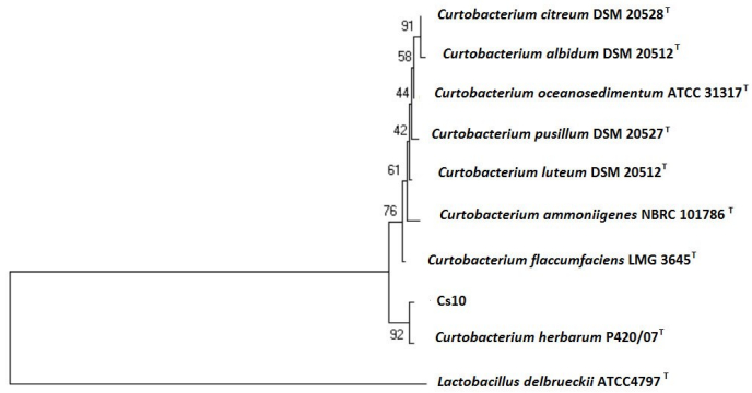
[36]	Ambardar S, Vakhlu J (2013) Plant growth promoting bacteria from Crocus sativus rhizosphere. World J Microbiol Biotechnol 29: 2271–2279. doi: 10.1007/s11274-013-1393-2
[37]	Tamura K, Dudley J, Nei M, et al. (2007) MEGA4: Molecular evolutionary genetics analysis (MEGA) software version 4.0. Mol Biol Evol 24: 1596–1599. doi: 10.1093/molbev/msm092
[38]	Peix A, Rivas-Boyero AA, Mateos PF, et al. (2001) Growth promotion of chickpea and barley by a phosphate solubilizing strain of Mesorhizobium mediterraneum under growth chamber conditions. Soil Biol Biochem 33: 103–110. doi: 10.1016/S0038-0717(00)00120-6
[39]	Alexander DB, Zuberer DA (1991) Use of chrome azurol S reagents to evaluate siderophore production by rhizosphere bacteria. Biol Fertil Soils 12: 39–45. doi: 10.1007/BF00369386
[40]	O'hara GW, Goss TJ, Dilworth MJ, et al. (1989) Maintenance of intracellular pH and acid tolerance in Rhizobium meliloti. Appl Environ Microbiol 55: 1870–1876.
[41]	Compant S, Reiter B, Sessitsch A, et al. (2005) Endophytic colonization of Vitis vinifera L. by plant growth-promoting bacterium Burkholderia sp. strain PsJN. Appl Environ Microbiol 71: 1685–1693.
[42]	Smalla K, Sessitsch A, Hartmann A (2006) The Rhizosphere: 'soil compartment influenced by the root'. FEMS Microbiol Ecol 56: 165–165. doi: 10.1111/j.1574-6941.2006.00148.x
[43]	Alves TMA, Kloos H, Zani CL (2003) Eleutherinone, a novel fungitoxic naphthoquinone from Eleutherine bulbosa (Iridaceae). Mem Inst Oswaldo Cruz 98: 709–712. doi: 10.1590/S0074-02762003000500021
[44]	Ifesan B, Ibrahim D (2010) Antimicrobial activity of crude ethanolic extract from Eleutherine americana. J Food Agric & Environ 8: 1233–1236.
[45]	Pearson WR (2014) BLAST and FASTA similarity searching for multiple sequence alignment, In: Multiple Sequence Alignment Methods, Human press, 75–101.
[46]	Hsieh TF, Huang HC, Mundel HH, et al. (2005) Resistance of common bean (Phaseolus vulgaris) to bacterial wilt caused by Curtobacterium flaccumfaciens pv. flaccumfaciens. J Phytopathol 153: 245–249. doi: 10.1111/j.1439-0434.2005.00963.x
[47]	Kim MK, Kim YJ, Kim HB, et al. (2008) Curtobacterium ginsengisoli sp. nov., isolated from soil of a ginseng field. Int J Syst Evol Microbiol 58: 2393–2397.
[48]	Behrendt U, Ulrich A, Schumann P, et al. (2002) Diversity of grass-associated Microbacteriaceae isolated from the phyllosphere and litter layer after mulching the sward; polyphasic characterization of Subtercola pratensis sp. nov., Curtobacterium herbarum sp. nov. and Plantibacter flavus gen. nov., sp. Int J Syst Evol Microbiol 52: 1441–1454.
[49]	Brian B (1977) Crocus sativus and its allies (Iridaceae). Plant Syst Evol 128: 89–103. doi: 10.1007/BF00985174
[50]	Alsayied NF, Fernández JA, Schwarzacher T, et al. (2015) Diversity and relationships of Crocus sativus and its relatives analysed by inter-retroelement amplified polymorphism (IRAP). Ann Bot 116: 359–368. doi: 10.1093/aob/mcv103
[51]	Rodríguez H, Fraga R, Gonzalez T, et al. (2007) Genetics of phosphate solubilization and its potential applications for improving plant growth-promoting bacteria, In: First International Meeting on Microbial Phosphate Solubilization, Dordrecht: Springer, 15–21.
[52]	Verma SC, Ladha JK, Tripathi AK (2001) Evaluation of plant growth promoting and colonization ability of endophytic diazotrophs from deep water rice. J Biotechnol 91: 127–141. doi: 10.1016/S0168-1656(01)00333-9
[53]	Kaur G, Reddy MS (2013) Phosphate solubilizing rhizobacteria from an organic farm and their influence on the growth and yield of maize (Zea mays L.). J Gen Appl Microbiol 59: 295–303.
[54]	Alikhani HA, Saleh-Rastin N, Antoun H (2007) Phosphate solubilization activity of rhizobia native to Iranian soils, In: First International Meeting on Microbial Phosphate Solubilization, Dordrecht: Springer, 35–41.
[55]	Ma Y, Prasad MNV, Rajkumar M, et al. (2011) Plant growth promoting rhizobacteria and endophytes accelerate phytoremediation of metalliferous soils. Biotechnol Adv 29: 248–258.
[56]	Navarro L, Dunoyer P, Jay F, et al. (2006) A plant miRNA contributes to antibacterial resistance by repressing auxin signaling. Science 312: 436–439.
[57]	Weilharter A, Mitter B, Shin MV, et al. (2011) Complete genome sequence of the plant growth-promoting endophyte Burkholderia phytofirmans strain PsJN. J Bacteriol 193: 3383–3384.
[58]	Taghavi S, Garafola C, Monchy S, et al. (2009) Genome survey and characterization of endophytic bacteria exhibiting a beneficial effect on growth and development of poplar trees. Appl Environ Microbiol 75: 748–757.
[59]	Kobayashi T, Nishizawa NK (2012) Iron uptake, translocation, and regulation in higher plants. Annu Rev Plant Biol 63: 131–152.
[60]	Crowley D (2006) Microbial siderophores in the plant rhizosphere. In: Iron nutrition in plants and rhizospheric microorganisms, Springer Netherlands, 169–198.
[61]	Schenk PM, Carvalhais LC, Kazan K (2012) Unraveling plant-microbe interactions: can multi-species transcriptomics help? Trends Biotechnol 30: 177–184. doi: 10.1016/j.tibtech.2011.11.002
[62]	Siebner-Freibach H, Hadar Y, Chen Y (2003) Siderophores sorbed on Ca-montmorillonite as an iron source for plants. Plant Soil 251: 115–124.
[63]	Verma VC, Singh SK, Prakash S (2011) Bio-control and plant growth promotion potential of siderophore producing endophytic Streptomyces from Azadirachta indica A. Juss. J Basic Microbiol 51: 550–556. doi: 10.1002/jobm.201000155

Reader Comments

Your name:*

Email:*
© 2017 the Author(s), licensee AIMS Press. This is an open access article distributed under the terms of the Creative Commons Attribution License (http://creativecommons.org/licenses/by/4.0)

通讯作者: 陈斌, bchen63@163.com

1.
沈阳化工大学材料科学与工程学院沈阳 110142

AIMS Microbiology

2.7 7.0

Metrics

Article views(6385) PDF downloads(1303) Cited by(18)

Preview PDF

Download XML

Export Citation

Article outline

Show full outline

AIMS Microbiology

Improvement of saffron production using Curtobacterium herbarum as a bioinoculant under greenhouse conditions

Related Papers:

Abstract

1. Introduction

2. Materials and methods

2.1. Data set

2.2. PSSM

2.3. AvBlock

2.4. DCT

2.5. DWT

2.6. HOG

2.7. PsePSSM

2.8. DRHGNN

2.8.1. Hypergraph learning statement

2.8.2. Hypergraph convolution

2.8.3. Residual hypergraph convolution

2.8.4. DRHGNN analysis

3. Results

3.1. Hyperparameter settings based on experience

3.2. Metrics

3.3. The selection of K value when constructing the hypergraph

3.4. Performance comparison of DRHGNN and HGNN with different layers

3.5. Performance comparison with multiple recently developed advanced methods

3.6. Stability analysis

3.7. Ablation study

4. Conclusions

Use of AI tools declaration

Acknowledgments

Conflict of interest

Data availability statement

References

Reader Comments

通讯作者: 陈斌, bchen63@163.com

Metrics

Figures and Tables

Other Articles By Authors

Related pages

Tools

Export File

Citation

Format

Content

Catalog

Abstract

1. Introduction

2. Materials and methods

2.1. Data set

2.2. PSSM

2.3. AvBlock

2.4. DCT

2.5. DWT

2.6. HOG

2.7. PsePSSM

2.8. DRHGNN

2.8.1. Hypergraph learning statement

2.8.2. Hypergraph convolution

2.8.3. Residual hypergraph convolution

2.8.4. DRHGNN analysis

3. Results

3.1. Hyperparameter settings based on experience

3.2. Metrics

3.3. The selection of K value when constructing the hypergraph

3.4. Performance comparison of DRHGNN and HGNN with different layers

3.5. Performance comparison with multiple recently developed advanced methods

3.6. Stability analysis

3.7. Ablation study

4. Conclusions

Use of AI tools declaration

Acknowledgments

Conflict of interest

Data availability statement

References