Sense of Community among Chinese Older Adults in the Greater Chicago Area: Findings from the PINE Study

1.   Introduction

Clustering analysis, artificial intelligence, neural networks and decision-making techniques are very famous for depicting vague and unreliable information in real-life problems. multi-attribute group decision making (MAGDM) procedures give important consideration to practical issues where the goal is to determine the best course of action rather than relying on a finite value in the presence of the different attributes. However, to process the vagueness in the information, the major theory of fuzzy sets (FSs) was presented by Zadeh ^[1] in 1965, in which he defined only the degree of membership (DoM), as $ \zeta :X\to \left[0, 1\right] $. FSs are one of the widely accepted theories to deal with MAGDM problems. Nevertheless, they have some limitations, as the theory of FSs neglected considering if an expert talked about the falsity information. Therefore, the theory of intuitionistic FSs (IFSs) was invented by Atanassov ^[2,3]. IFSs have a DoM "$ \zeta :X\to \left[0, 1\right] $" and degree of non-membership (DoNM) "$ \delta :X\to \left[0, 1\right] $" with the restriction $ 0\le sum\left(\zeta \left(x\right), \delta \left(x\right)\right)\le 1 $. Some recent work on the theory and applications of IFSs is discussed in ^[4,5,6]. Other works discuss Pythagorean FSs (PyFSs) ^[7], a decision-making problem ^[8,9,10,11], q-rung orthopair FSs (qROFSs) ^[12] and their applications in decision-making problems ^{[13,14,15,16,17]}.

FSs and IFSs are unable to meet the requirements when dealing with conclusions that involve multiple forms of responses, such as yes, no, abstain and refusal. The notion of an IFS has a strict condition, and it does not provide independence in assigning the DoM and DoNM and binds their sum between $ 0 $ and $ 1 $. To deal with the above types of situations, the major idea of picture FSs (PFSs) was derived by Cuong ^[18]. They are more suitable than the theories of FSs or IFSs in dealing with this lack of data. PFSs are represented by the DoM, abstinence (DoA) and DoNM with a valuable condition: $ 0\le sum\left(\zeta \left(x\right), \vartheta \left(x\right), \delta \left(x\right)\right)\le 1 $. Furthermore, the theory of PFSs is more suitable and reliable as compared to FSs and IFSs for evaluating uncertainty and ambiguous types of data. Various researchers started working on PFSs as soon as they were developed. Numberless research on PFSs can be seen in ^{[19,20,21,22]}. From the above analysis, we noticed that every expert or decision-maker has faced the following three major issues during the decision-making process:

1) How do we collect the information on a suitable scale to state the data?

2) How do we aggregate the collection of a finite number of attributes into a singleton set?

3) How do we determine the best decision using the theory of score information?

Therefore, this research examines the prioritized Aczel-Alsina averaging and geometric AOs based on the concept of PF information. Menger ^[23] presented the concept of triangular norms, and it was discovered that the norms' operations played a very important role in the field of FS theory. Since then, many scholars have extended the theory of triangular norms, such as the Hamacher t-norm and t-conorm ^[24], spherical t-norm and t-conorm ^[25], Einstein t-norm and t-conorm ^[26], Archimedean t-norm and t-conorm ^[27], Frank t-norm and t-conorm ^[28,29]. In the last few years, Klement et al. ^[18] studied more efficiently related properties of triangular norms and their corresponding features.

The concept of Aczel-Alsina t-norm and t-conorm was proposed by Aczel and Alsina ^[30], which has the ability of changeability with the condition of limitation. The Aczel-Alsina t-norm and t-conorm were derived in 1982, and they are modified forms of the algebraic t-norm and t-conorm. After successfully constructing this information, various scholars have utilized it in different areas. For example, Senapati et al. ^[31,32] created Aczel-Alsina AOs for interval-valued IFSs (IVIFSs) and a structure of IFSs, and they then used them to address the MADM difficulties. Furthermore, Senapati ^[33] considered Aczel-Alsina AOs based on PFSs with application to MADM. The concept of T-spherical fuzzy Aczel Alsina AOs and Pythagorean F aczel alsina AOs were presented by Hussain et al. ^[34,35] to solve MADM problems. From our point of view, we noticed that the theory of Aczel-Alsina AOs is very valuable and reliable because of their structure. Moreover, developing the theory of Aczel-Alsina aggregation based on prioritized information for managing the theory of PF data is a very ambiguous and awkward task for scholars, because no one can derive it before. The major advantages of the presented theory are listed below:

1) Aczel-Alsina AOs based on FSs, IFSs and PFSs are the special cases of the proposed work if we removed the prioritized information from the derived theory.

2) Prioritized AOs based on FSs, IFSs and PFSs are the special cases of the proposed work if we used the algebraic operational laws instead of Aczel-Alsina operational laws in the derived theory.

3) Prioritized Aczel-Alsina AOs based on FSs and IFSs are the special cases of the proposed work if we removed the neural or abstinence information from the derived theory.

The theory of Aczel-Alsina AOs based on prioritized degree for managing the theory of PFSs is very valuable and dominant. Because of this construction, we evaluate a lot of real-life problems, and the proposed theory has not been presented by anyone yet. Numerous situations that occur frequently in daily life require the use of a mathematical function that may reduce a series of data into a single value. The investigation of AO has a big impact on MADM issues. In recent years, a lot of researchers have worked on how to aggregate data because of its extensive use in various sectors. However, there are several situations where the data that need to be aggregated in terms of prioritization have a strict relationship. In this research, we focus on the MADM problem with a priority relationship between the criteria. Different priority levels apply to the criteria. Take the situation where we wish to purchase some land, to construct a house based on utility access ($ {C}_{1} $), site ($ {C}_{2} $) and pricing ($ {C}_{3} $). We are not interested in paying for utility access based on cost and location. That is, there is strict prioritization among the parameters in this scenario, where > denotes "is preferable to." To address the MADM issue that was previously prioritized, Yager ^[36] introduced several AOs, including the prioritized scoring (PS) operator. Three operators, the prioritized "and" operator, the prioritized "or" and the prioritized averaging (PA) operator, . The prioritized OWA (POWA) operator, based on the BUM function, was also proposed by Yager ^[37]. A prioritized weighted AO based on the OWA operator and triangle norms (t-norms) was proposed by Yan et al. ^[38]. Inspired by the above analysis, the main contributions of this research are listed below:

1) Analyzing the theory of averaging and geometric AOs in the presence of the Aczel-Alsina operational laws and prioritization degree based on PF information, such as the prioritized PF Aczel-Alsina averaging (PPFAAA) operator and prioritized PF Aczel-Alsina geometric (PPFAAG) operator

2) Examining properties such as idempotency, monotonicity and boundedness for the derived operators and also evaluating some important results

3) Using the derived operators to create a system for controlling the MAGDM problem using PF information

4) Showing the approach's effectiveness and the developed operators' validity with a numerical example

5) Comparing the proposed work with a few existing operators are also listed in this manuscript

The remainder of this paper is designed as follows: In Section 2, we introduce the concept of PPFs and their special cases. The objective of Section 3 is to introduce the concept of the PPFAAA operator and PPFAAG operator. In Section 4, we define a method of MAGDM by using the PPFAAA and PPFAAG operators to solve algebraic issues. In Section 5, we study the impact of the parameter by using various values of $ \eta $. In Section 6, we compare the proposed work with the previously defined methods. In the last section, we conclude this research paper with a few comments.

2.   Preliminaries

The proposed work is introduced in this part using some fundamental ideas. We can better understand this article with the help of these concepts. The terms PFS, Aczel-Alsina triangular norm(TN) and triangular conorm(TCN) are defined here.

Definition 1. ^[39] On a non-empty set $ X $, a PFS is of the shape

Here, $ \zeta, \vartheta, \delta :X\to \left[0, 1\right] $ denote the DoM, DoA and DoNM, respectively. Further, $ r\left(x\right) = 1-sum\left(\zeta \left(x\right), \vartheta \left(x\right), \delta \left(x\right)\right) $ represents the DoR of $ x\in X $, and the triplet $ \left(\zeta, \vartheta, \delta \right) $ is termed a picture fuzzy value (PFV).

The basic set-theoretic operations of union, intersection, inclusion and complement of PFVs were also proposed by Cuong ^[18] and are given as follows.

Definition 2. ^[18] Let $ \varrho = \left(\zeta, \vartheta, \delta \right), {\varrho }_{1} = \left({\zeta }_{1}, {\vartheta }_{1}, {\delta }_{1}\right) $ and $ {\varrho }_{2} = \left({\zeta }_{2}, {\vartheta }_{2}, {\delta }_{2}\right) $ be three PFVs. Then,

Definition 3. Let $ \varrho = \left(\zeta, \vartheta, \delta \right) $ be a PFV. Then, the score value of $ \varrho $ is defined as

The score function for PFVs is given as

Definition 4. ^[18] Let $ \varrho = \left(\zeta, \vartheta, \delta \right) $ be PFVs. Then, the score values of $ \varrho $ are defined as

Because of these score functions, for two PFVs $ {\varrho }_{1} = \left({\zeta }_{1}, {\vartheta }_{1}, {\delta }_{1}\right) $ and $ {\varrho }_{2} = \left({\zeta }_{2}, {\vartheta }_{2}, {\delta }_{2}\right) $, we have

$ {\varrho }_{1} $ is superior to $ {\varrho }_{2} $ if $ SC\left({\varrho }_{1}\right) > SC\left({\varrho }_{2}\right) $.

$ {\varrho }_{1} $ is inferior to $ {\varrho }_{2} $ if $ SC\left({\varrho }_{1}\right) < SC\left({\varrho }_{2}\right) $.

In the case when $ SC\left({\varrho }_{1}\right) = SC\left({\varrho }_{2}\right) $, two PFVs can be distinguished from each other with the help of the accuracy function, which is defined as follows:

Definition 5. ^[18] Let $ \varrho = \left(\zeta, \vartheta, \delta \right) $ be a PFVs. Then, the accuracy value of $ \varrho $ is defined as

Because of the accuracy function, for PFVs $ {\varrho }_{1} = \left({\zeta }_{1}, {\vartheta }_{1}, {\delta }_{1}\right) $ and $ {\varrho }_{2} = \left({\zeta }_{2}, {\vartheta }_{2}, {\delta }_{2}\right) $, we have

$ {\varrho }_{1} $ is superior to $ {\varrho }_{2} $ if $ AC\left({\varrho }_{1}\right) > AC\left({\varrho }_{2}\right) $.

$ {\varrho }_{1} $ is inferior to $ {\varrho }_{2} $ if $ AC\left({\varrho }_{1}\right) < AC\left({\varrho }_{2}\right) $.

$ {\varrho }_{1} $ is similar to $ {\varrho }_{2} $ if $ AC\left({\varrho }_{1}\right) = AC\left({\varrho }_{2}\right) $.

Definition 6. ^[33] Let $ \varrho = \left(\zeta, \vartheta, \delta \right), {\varrho }_{1} = \left({\zeta }_{1}, {\vartheta }_{1}, {\delta }_{1}\right) $ and $ {\varrho }_{2} = \left({\zeta }_{2}, {\vartheta }_{2}, {\delta }_{2}\right) $ be three PFVs where $ л\ge 1 $ and $ \eta > 0 $. Then, Aczel-Alsina operations of PFVs are defined by

3.   Picture fuzzy prioritized Aczel-Alsina aggregation operators

In this section, we analyze the theory of averaging and geometric AOs in the presence of the Aczel-Alsina operational laws and prioritization degree based on PF information, such as the PPFAAA operator and PPFAAG operator. Moreover, we examine properties such as idempotency, monotonicity and boundedness for the derived operators and also evaluated some important results.

Definition 7. Let $ {\varrho }_{n} = \left(n = \mathrm{1, 2}, 3\dots h\right) $ be several PFVs. Then, the PFPAAA operator is a mapping $ {\varrho }^{n}\to \varrho $ defined by

Therefore, using the Aczel-Alsina operations on PFVs, we proposed the following theorem.

Theorem 1. Let $ {\varrho }_{n} = \left({\zeta }_{n}, {\vartheta }_{n}, {\delta }_{n}\right)(n = \mathrm{1, 2}, 3\dots h) $ be an accumulation of PFVs. Then, the accumulated value of their employing the PFPAAA operation is indeed a PFV, as

The proof of Theorem 1 is given in Appendix A.

Theorem 2. (Idempotency). If all $ {\varrho }_{n} = \left({\zeta }_{n}, {\vartheta }_{n}, {\delta }_{n}\right)(n = \mathrm{1, 2}, 3\dots h) $ are equal, that is, $ {\varrho }_{n} = \varrho $ for all n, then

The proof of Theorem 2 is given in Appendix B.

Theorem 3. (Boundedness). Let $ {\varrho }_{n} = \left({\zeta }_{n}, {\vartheta }_{n}, {\delta }_{n}\right)(n = \mathrm{1, 2}, 3\dots h) $ be an accumulation of PFVs. Let $ {\varrho }^{-} = min\left({\varrho }_{1}, {\varrho }_{2}, \dots {\varrho }_{n}\right) $ and $ {\varrho }^{+} = max\left({\varrho }_{1}, {\varrho }_{2}, \dots {\varrho }_{h}\right) $. Then, we have

The proof of Theorem 3 is given in Appendix C.

Theorem 4. (Monotonicity) Let $ {\varrho }_{n} $ and $ {{\varrho }_{n}}^{'}(n = \mathrm{1, 2}, 3\dots h) $ be two sets of PFVs. If $ {\varrho }_{n}\le {{\varrho }_{n}}^{'} $ for all n, then

Theorem 5. Let $ {\varrho }_{n} = \left({\zeta }_{n}, {\vartheta }_{n}, {\delta }_{n}\right)(n = \mathrm{1, 2}, 3\dots h) $ be an accumulation of PFVs, $ {T}_{n} = {\prod }_{n = 1}^{h-1}S\left({\varrho }_{h}\right)\left(n = \mathrm{2, 3}, \dots h\right), {T}_{1} = 1 $, and $ S\left({\varrho }_{h}\right) $ is the score of PFVs $ {\varrho }_{h} $ if $ \psi = \left(\mu, \phi, \nu \right) $ is an IVPFV on $ X $, then

The proof of Theorem 5 is given in Appendix D.

Theorem 6. Let $ {\varrho }_{n} = \left({\zeta }_{n}, {\vartheta }_{n}, {\delta }_{n}\right)\left(n = \mathrm{1, 2}, 3\dots h\right) $ be a collection of PFVs.$ {T}_{n} = {\prod }_{n = 1}^{h-1}S\left({\varrho }_{h}\right)\left(n = \mathrm{2, 3}, \dots h\right), $ $ {T}_{1} = 1 $, and $ S\left({\varrho }_{h}\right) $ be the score of PFVs $ {\varrho }_{n} $ if $ r > 0 $, PFV on $ X $. Then,

The proof of Theorem 6 is given in Appendix E.

Theorem 7. Let $ {\varrho }_{n} = \left({\zeta }_{n}, {\vartheta }_{n}, {\delta }_{n}\right)\left(n = \mathrm{1, 2}, 3\dots h\right) $ be a collection of PFVs. Let $ {T}_{n}{\prod }_{n = 1}^{h-1}S\left({\varrho }_{h}\right) $ $ \left(n = \mathrm{2, 3}, \dots h\right), {T}_{1} = 1 $, and $ S\left({\varrho }_{h}\right) $ be the score of PFVs $ {\varrho }_{n} $ if $ r > 0 $, $ \psi = \left(\mu, \phi, \nu \right) $ is a PFV on $ X $. Then,

The proof of Theorem 7 is given in Appendix F.

Theorem 8. Let $ {\varrho }_{n} = \left({\zeta }_{n}, {\vartheta }_{n}, {\delta }_{n}\right) $ and $ \psi = \left({\mu }_{n}, {\phi }_{n}, {\nu }_{n}\right)(n = \mathrm{1, 2}, 3\dots h) $ be a collection of PFVs. $ {T}_{n} = {\prod }_{n = 1}^{h-1}S\left({\varrho }_{h}\right)\left(n = \mathrm{2, 3}, \dots h\right), {T}_{1} = 1 $, and $ S\left({\varrho }_{n}\right) $ be the score of PFVs $ {\varrho }_{n} $ if $ r > 0 $, is a PFV on $ X $.

Then,

The proof of Theorem 8 is given in Appendix G.

Definition 8. Let $ {\varrho }_{n} = \left(n = \mathrm{1, 2}, 3\dots h\right) $ be a collection of several PFVs. Then, the PFPAAG operator is a mapping $ {\varrho }^{n}\to \varrho $ defined by

Therefore, using the Aczel-Alsina operations on PFVs, we obtain the following theorem.

Theorem 9. Let $ {\varrho }_{n} = \left({\zeta }_{n}, {\vartheta }_{n}, {\delta }_{n}\right)(n = \mathrm{1, 2}, 3\dots h) $ be an accumulation of PFVs. Then, the accumulated value of them employing the PFPAAG operation is indeed PFVs, such as

Proof. The proof is similar to Theorem 1.

Theorem 10. (Idempotency). If all $ {\varrho }_{n} = \left({\zeta }_{n}, {\vartheta }_{n}, {\delta }_{n}\right)(n = \mathrm{1, 2}, 3\dots h) $ are equal, that is, $ {\varrho }_{n} = \varrho $, for all

n, then we have

Proof. The proof is similar to Theorem 2.

Theorem 11. (Boundedness). Suppose $ {\varrho }_{n} = \left({\zeta }_{n}, {\vartheta }_{n}, {\delta }_{n}\right)(n = \mathrm{1, 2}, 3\dots h) $ is an accumulation of PFVs.

Let $ {\varrho }^{-} = min\left({\varrho }_{1}, {\varrho }_{2}, \dots {\varrho }_{n}\right) $ and $ {\varrho }^{+} = max\left({\varrho }_{1}, {\varrho }_{2}, \dots {\varrho }_{h}\right) $. Then, we have

Proof. The proof is similar to Theorem 3.

Theorem 12. Suppose $ {\varrho }_{n} = \left({\zeta }_{n}, {\vartheta }_{n}, {\delta }_{n}\right)(n = \mathrm{1, 2}, 3\dots h) $ is an accumulation of PFVs, $ {T}_{n} = {\prod }_{n = 1}^{h-1}S\left({\varrho }_{h}\right)\left(n = \mathrm{2, 3}, \dots h\right), {T}_{1} = 1 $, and $ S\left({\varrho }_{h}\right) $ be the score of PFVs $ {\varrho }_{n} $ if $ \psi = \left(\mu, \phi, \nu \right) $ is an PFVs on X, then

Proof. The proof is similar to Theorem 4.

Theorem 13. Suppose $ {\varrho }_{n} = \left({\zeta }_{n}, {\vartheta }_{n}, {\delta }_{n}\right)\left(n = \mathrm{1, 2}, 3\dots h\right) $ is a collection of PFVs.$ {T}_{n} = {\prod }_{n = 1}^{h-1}S\left({\varrho }_{h}\right)\left(n = \mathrm{2, 3}, \dots h\right), {T}_{1} = 1 $, and $ S\left({\varrho }_{h}\right) $ be the score of PFVs $ {\varrho }_{n} $ if $ r > 0 $ PFVs on $ X, $ then we have

Proof. The proof is similar to Theorem 5.

Theorem 14. Let $ {\varrho }_{n} = \left({\zeta }_{n}, {\vartheta }_{n}, {\delta }_{n}\right)(n = \mathrm{1, 2}, 3\dots h) $ be a collection of PFVs. $ {T}_{n} = {\prod }_{n = 1}^{h-1}S\left({\varrho }_{h}\right)\left(n = \mathrm{2, 3}, \dots h\right), {T}_{1} = 1 $, and $ S\left({\varrho }_{h}\right) $ be the score of PFVs $ {\varrho }_{n} $ if $ r > 0 $, $ \psi = \left(\mu, \phi, \nu \right) $ is a PFV on $ X $. Then, we have

Proof. The proof is similar to Theorem 6.

Theorem 15. Let $ {\varrho }_{n} = \left({\zeta }_{n}, {\vartheta }_{n}, {\delta }_{n}\right)(n = \mathrm{1, 2}, 3\dots h) $ be a collection of PFVs. $ {T}_{n} = {\prod }_{n = 1}^{h-1}S\left({\varrho }_{h}\right)\left(n = \mathrm{2, 3}, \dots h\right), {T}_{1} = 1 $, and $ S\left({\varrho }_{h}\right) $ be the score of PFVs $ {\varrho }_{n} $ if $ r > 0 $, $ \psi = \left(\mu, \phi, \nu \right) $ is a PFV on $ X $. Then, we have

Proof. The proof is similar to Theorem 7.

Theorem 16. Suppose $ {\varrho }_{n} = \left({\zeta }_{n}, {\vartheta }_{n}, {\delta }_{n}\right) $, and $ \psi = \left({\mu }_{n}, {\phi }_{n}, {\nu }_{n}\right)(n = \mathrm{1, 2}, 3\dots h) $ is a collection of PFVs. $ {T}_{n} = {\prod }_{n = 1}^{h-1}S\left({\varrho }_{h}\right)\left(n = \mathrm{2, 3}, \dots h\right), {T}_{1} = 1 $, and $ S\left({\varrho }_{h}\right) $ be the score of PFVs $ {\varrho }_{n} $ if $ r > 0 $, is a PFV on $ X $. Then we have

Proof. The proof is similar to Theorem 8.

4.   MAGDM based on derived operators

We will create a MAGDM methodology in this section based on the picture fuzzy environment to illustrate reliability and effectiveness. In this problem, assume that $ x = \left\{{x}_{1}, {x}_{2}, {x}_{3}\dots {x}_{m}\right\} $ is the set of attributes and that the attributes are ranked in order of alternatives, with $ C = \left\{{C}_{1}, {C}_{2}, {C}_{3}\dots {C}_{z}\right\} $ priority as indicated by the linear ordering $ {C}_{1} > {C}_{2} > {C}_{3}\dots > {C}_{z} $. If $ j < i $, and $ E = \left\{{e}_{1}, {e}_{2}, {e}_{3}\dots {e}_{p}\right\} $ is the set of decision-makers, then $ {C}_{j} $ has a higher priority than $ {C}_{i} $. If $ \varsigma < \tau $, then there is a prioritization between the decision makers expressed by the linear ordering $ {e}_{1} > {e}_{2} > {e}_{3}\dots > {e}_{z} $ indicating that $ {e}_{\varsigma } $ has a higher priority than $ {e}_{\tau } $ if $ \varsigma < \tau $. $ \mathrm{{\rm K}} = {\left({K}_{ij}^{q}\right)}_{nxm} $ is a picture valued Aczel-Alsina decision matrix, and $ {K}_{ij}^{q} = \left({\zeta }^{q}, {\vartheta }^{q}, {\delta }^{q}\right) $ is an attribute value provided by the decision maker $ {e}_{q} $ which is expressed in a PFPAAA, where $ \zeta $ indicates the degree that the alternative $ {y}_{i} $ satisfies the attribute $ {C}_{j} $ expressed by the decision maker $ {e}_{q}, {\delta }^{q} $ indicate the degree that the alternative $ {y}_{i} $ does not satisfy the attribute $ {C}_{j} $ expressed by the decision maker $ {e}_{q} $, and $ {\vartheta }^{q} $ is the degree about which the decision maker has some doubts. If all the attributes $ {C}_{j}(\mathrm{1, 2}, 3\dots m) $ are the same type, then the attribute value does not need normalization. Otherwise, we normalize the decision-maker matrix $ {{\rm K}}^{q} = {\left({K}_{ij}^{q}\right)}_{nxm} $ into $ {\mathrm{R}}^{q} = {\left({K}_{ij}^{q}\right)}_{nxm} $ where

where $ {\overline {K}}_{ij}^{q} $ is the complement of $ {K}_{ij}^{q} $ such that $ {\overline {K}}_{ij}^{q} = \left({\omega }^{q}, {\alpha }^{q}, {\beta }^{q}\right) $ and $ {r}_{ij}^{q} = ({\alpha }^{q}, {\beta }^{q}, {\omega }^{q}) $ $ i = \mathrm{1, 2}, 3\dots, m, j = \mathrm{1, 2}, 3\dots, z $

Then, we utilized the PFPAAA operator to develop an approach to multi-criteria decision-making under PFVs; the following are the key steps:

Step 1: By using the following equations, determine the values of $ {T}_{ij}^{q}\left(q = \mathrm{1, 2}, 3\dots s\right) $:

Step 2: By using the PFPAAA operator,

By using the PFPAAG operator,

To aggregate the decision-making of each PFV $ {\mathrm{R}}^{q} = {\left({r}_{ij}^{q}\right)}_{nxm}\left(q = \mathrm{1, 2}, 3\dots s\right) $ into the decision-making of collective PFVs $ {\mathrm{R}}^{q} = {\left({r}_{ij}^{q}\right)}_{nxm}i = \mathrm{1, 2}, 3\dots, m $, $ j = \mathrm{1, 2}, 3\dots, z $.

Step 3: Evaluate the values of $ {T}_{ij} $ $ \left(i = \mathrm{1, 2}, 3\dots, m\ \ \ j = \mathrm{2, 3}\dots, s\right) $ based on the following equations:

Step 4: Aggregate the PFVs $ {r}_{ij} $ for each alternative $ {x}_{i} $ by PFPAAA operator

Or

Step 5: Rank all the alternatives by the score function described in section 2.

Then, the bigger the value of $ S\left({r}_{i}\right) $ is, the larger the overall PFPAAA $ {r}_{i} $, and thus the alternative $ {k}_{i}\left(i = \mathrm{1, 2}, 3\dots m\right) $.

5.   Practical application

The best car selection issue of a person wanting to purchase a car among different vehicles in the same category is resolved in this research using the multi-attribute decision-making method. Every car has an automatic transmission and runs on gasoline. First, the criteria for the best automobile selection problem are established by doing a literature search and taking into account the views of the prospective buyer. The criteria are determined as follows based on the information obtained: engine capacity, fuel usage, post-purchase support and comfort. A panel of decision-makers estimate the performance and select the best to attain the most benefits among the set of alternatives $ s = \left\{{s}_{1}, {s}_{2}, {s}_{3}, {s}_{4}\right\} $. The following criteria are used to determine the steps of the algorithm under consideration.

The attribute values do not require normalization, and therefore, $ {R}^{q} = {D}^{q} = {\left({d}_{ij}^{q}\right)}_{5\times 4} = {\left({r}_{ij}^{q}\right)}_{5\times 4} $.

The main steps are listed below according to the PFPAAA operator:

Step 1: Find the values of $ {T}_{ij}^{1}, {T}_{ij}^{2}, {T}_{ij}^{3} $.

Step 2: Use the PFPAAA operator, Eq (8), to combine each PFVs decision making $ {R}^{q} = {\left({r}_{ij}^{q}\right)}_{5\times 4}(q = \mathrm{1, 2}, 3) $ into a collective picture fuzzy decision matrix $ \widetilde {R} = {\left(\widetilde {{r}_{ij}}\right)}_{5X4} $.

Step 3: By using Eqs (19) and (20), find the values of $ {T}_{ij}\left(i = \mathrm{1, 2}, 3\dots, m\ \ \ j = \mathrm{1, 2}, 3\dots, z\right) $.

Step 4: Utilize the PFPAAA operator to aggregate all the preference values $ {r}_{ij}\left(i = \mathrm{1, 2}, \mathrm{3, 4}, 5\right) $ in the ith line of $ \widetilde {R} $ and get the overall preference values $ {r}_{i} $:

Step 5: Calculate the scores of $ {r}_{i}\left(i = \mathrm{1, 2}, \mathrm{3, 4}, 5\right) $, respectively:

Since

we have

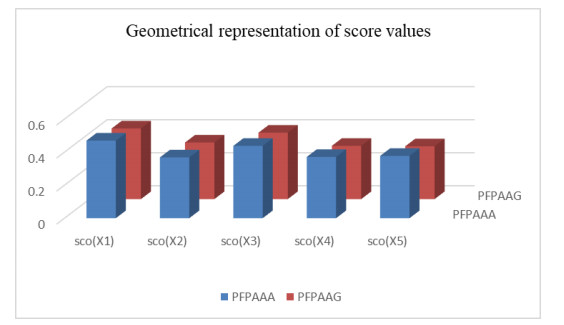
Therefore, $ {x}_{1} $ is the best option.

By using PFPAAG operators, these are the primary steps:

Step 1: Check step 1.

Step 2: Use the PFPAAG operators to calculate all the PFVs' decision making values $ \widetilde {R} = {\left({\widetilde {r}}_{ij}^{'}\right)}_{5X4}(q = \mathrm{1, 2}, 3) $ into a collective picture fuzzy decision matrix $ \widetilde {{R}^{'}} = {\left({\widetilde {r}}_{ij}^{'}\right)}_{5X4}(q = \mathrm{1, 2}, 3) $.

Step 3: Aggregate the values of $ {T}_{ij}^{'}\left(i = \mathrm{1, 2}, 3\dots, m\ \ \ j = \mathrm{1, 2}, 3\dots, z\right) $ based on Eqs (19) and (20).

Step 4: Utilize the PFPAAA operator to aggregate all the preference values $ {r}_{ij}^{'}\left(i = \mathrm{1, 2}, \mathrm{3, 4}, 5\right) $ in the ith line of $ \widetilde {{R}^{'}} $, and get the overall preference values $ {r}_{ij}^{'} $:

Step 5: Calculate the scores of $ {r}_{i}\left(i = \mathrm{1, 2}, \mathrm{3, 4}, 5\right) $, respectively:

Since

we have

Therefore, $ {x}_{2} $ is the best option. Thus, the different rankings of alternatives are obtained by the PFPAAA and PFPAAG operators.

6.   Comparative analysis

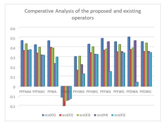
Comparative analysis is one of the most valuable and dominant techniques for evaluating the supremacy between any two different kinds of operators. We compared the proposed theory with some existing operators: the picture fuzzy weighted averaging (PFWA) operator, proposed by Wei ^[40]; the picture fuzzy weighted geometric (PFWG) operator, invented by Wei ^[40]; the picture fuzzy hybrid weighted averaging (PFHWA) operator, derived by Wei ^[39]; the picture fuzzy hybrid weighted geometric (PFHWG) operator, presented by Wei ^[39]; the picture fuzzy frank weighted averaging (PFFWA) operator, discovered by Seikh et al. ^[28]; the picture fuzzy frank weighted geometric (PFFWG) operator, presented by Seikh et al. ^[28]; the picture fuzzy Dombi weighted averaging (PFDWA) operator, examined by Jana et al. ^[41]; and the picture fuzzy Dombi weighted geometric (PFDWG) operator, evaluated by Jana et al. ^[41].

The comparison is summarized in Table 5. Using the data in Table 4, make a side-by-side comparison of the proposed and current operators. As can be seen from the analysis, the best candidate for both ways is $ {S}_{1} $ by using PFPAAA and PFPAAG AOs, and the rankings for both methods are equal. This confirms the approach we recommended in this article is logical and efficient. The TN and TCN used by Aczel-Alsina are more flexible than those used by other AOs. The main benefit of the PFPAAA and PFPAAG operators we presented is that they introduce a prioritized relationship structure of prioritized aggregating operators, which allows us to represent the prioritized relationships more accurately between attributes. However, the alternative suggested by others does not consider such real-world circumstances where some attributes may have higher priority than other attributes.

7.   Conclusions

The main contributions of this research are listed below:

1) We analyzed the theory of averaging and geometric AOs in the presence of the Aczel-Alsina operational laws and prioritization degree based on PF information, such as the PPFAAA operator and PPFAAG operator.

2) We examined properties such as idempotency, monotonicity and boundedness for the derived operators and also evaluated some important results.

3) We used the derived operators to create a system for controlling the MAGDM problem using PF information.

4) We showed the approach's effectiveness and the developed operators' validity, and a numerical example has been given.

5) We compared the proposed work with a few existing operators listed in this manuscript.

6) We shall try to utilize the abovementioned method in the future and expand its application to various fuzzy situations.

Appendix

Appendix A

Proof. Through the method of mathematical induction, we are ready to prove Theorem 1 as follows: In the context of $ n = 2 $ and the PFV Aczel-Alsina operations, we obtain

We obtain

As a result, $ n = 2 $ (15) holds $. $ Furthermore, we assume that for $ n = k $ (15), we obtain

Now, for $ n = k+1 $,

Thus, Eq 15 is correct for $ n = k+1 $. Consequently, we conclude that Eq 15 is true for n.

Appendix B

Proof. Since $ {\varrho }_{n} = \left({\zeta }_{n}, {\vartheta }_{n}, {\delta }_{n}\right) = \varrho (n = \mathrm{1, 2}, 3\dots h) $, by Eq 15, we have

Thus, $ $

Appendix C

Proof. Let $ {\varrho }^{-} = min\left({\varrho }_{1}, {\varrho }_{2}, \dots {\varrho }_{n}\right) = \left({\zeta }^{-}, {\vartheta }^{-}, {\delta }^{-}\right) $ and $ {\varrho }^{+} = max\left({\varrho }_{1}, {\varrho }_{2}, \dots {\varrho }_{n}\right) = \left({\zeta }^{+}, {\vartheta }^{+}, {\delta }^{+}\right) $. As a result, we get the inequalities that follow,

Therefore,

Appendix D

Proof. Let

According to Theorem 1, we have

By utilizing the operational laws of PFVs, we obtain

Thus,

Appendix E

Proof. Following the operational rules listed in Section 2, we get

According to Theorem 1, we have

Thus,

Appendix F

Proof.

Thus,

Appendix G

Proof. We have

Thus,