Influence of network structure on infectious disease control

Nariyuki Nakagiri; Hiroki Yokoi; Yukio Sakisaka; Kei-ichi Tainaka; Kazunori Sato; Nariyuki Nakagiri; Hiroki Yokoi; Yukio Sakisaka; Kei-ichi Tainaka; Kazunori Sato

doi:10.3934/mbe.2025034

Mathematical Biosciences and Engineering

2025, Volume 22, Issue 4: 943-961. doi: 10.3934/mbe.2025034

Previous Article Next Article

Research article Special Issues

Influence of network structure on infectious disease control

1.
School of Human Science and Environment, University of Hyogo, Himeji 670-0092, Japan
2.
Fisheries Resources Institutes (FRI), Japan Fisheries Research and Education Agency, 2-14-4 Fukuura, Kanazawa, Yokohama, Kanagawa 236-8648, Japan
3.
Division of Early Childhood Care and Education, Nakamura Gakuen University Junior College, Fukuoka, 814-0198, Japan
4.
Department of Mathematical and Systems Engineering, Shizuoka University, Hamamatsu 432-8561, Japan

Academic Editor: Ruijun Zhao

Received: 08 October 2024 Revised: 20 February 2025 Accepted: 27 February 2025 Published: 12 March 2025

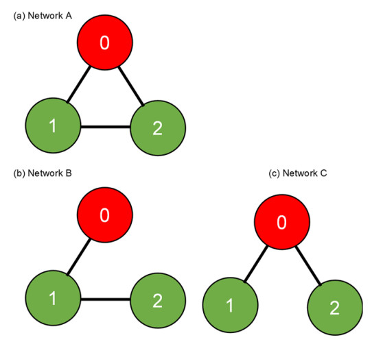
Control of infectious disease is very hard but important for the life of human beings. We study the susceptible–infected–susceptible (SIS) model of three-city networks. The SIS model simply contains both infection and recovery processes. We assume that human beings ("agents") live in three spatially separated cities, and they randomly migrate between cities. Two methods are applied: one is a computer simulation of an agent-based model, and the other is the theory of metapopulation dynamics. Both the simulation and theory reveal that the "hub city" plays an important role for disease control. It was found that we can eliminate the entire infection by disease control measures on the hub city only. Moreover, we found a paradoxical result: increased agent interaction does not necessarily lead to the spread of infection.

Keywords:

Citation: Nariyuki Nakagiri, Hiroki Yokoi, Yukio Sakisaka, Kei-ichi Tainaka, Kazunori Sato. Influence of network structure on infectious disease control[J]. Mathematical Biosciences and Engineering, 2025, 22(4): 943-961. doi: 10.3934/mbe.2025034

Related Papers:

[1]	Jun Hyung Bae, Sang-Mook Lee . Investigation of SIS epidemics on dynamic network models with temporary link deactivation control schemes. Mathematical Biosciences and Engineering, 2022, 19(6): 6317-6330. doi: 10.3934/mbe.2022295
[2]	Joan Ponce, Horst R. Thieme . Can infectious diseases eradicate host species? The effect of infection-age structure. Mathematical Biosciences and Engineering, 2023, 20(10): 18717-18760. doi: 10.3934/mbe.2023830
[3]	Liqiong Pu, Zhigui Lin . A diffusive SIS epidemic model in a heterogeneous and periodically evolvingenvironment. Mathematical Biosciences and Engineering, 2019, 16(4): 3094-3110. doi: 10.3934/mbe.2019153
[4]	Yicang Zhou, Zhien Ma . Global stability of a class of discrete age-structured SIS models with immigration. Mathematical Biosciences and Engineering, 2009, 6(2): 409-425. doi: 10.3934/mbe.2009.6.409
[5]	Xin-You Meng, Tao Zhang . The impact of media on the spatiotemporal pattern dynamics of a reaction-diffusion epidemic model. Mathematical Biosciences and Engineering, 2020, 17(4): 4034-4047. doi: 10.3934/mbe.2020223
[6]	Junbo Jia, Zhen Jin, Lili Chang, Xinchu Fu . Structural calculations and propagation modeling of growing networks based on continuous degree. Mathematical Biosciences and Engineering, 2017, 14(5&6): 1215-1232. doi: 10.3934/mbe.2017062
[7]	Zhen Jin, Guiquan Sun, Huaiping Zhu . Epidemic models for complex networks with demographics. Mathematical Biosciences and Engineering, 2014, 11(6): 1295-1317. doi: 10.3934/mbe.2014.11.1295
[8]	Andreas Widder, Christian Kuehn . Heterogeneous population dynamics and scaling laws near epidemic outbreaks. Mathematical Biosciences and Engineering, 2016, 13(5): 1093-1118. doi: 10.3934/mbe.2016032
[9]	Abhishek Savaliya, Rutvij H. Jhaveri, Qin Xin, Saad Alqithami, Sagar Ramani, Tariq Ahamed Ahanger . Securing industrial communication with software-defined networking. Mathematical Biosciences and Engineering, 2021, 18(6): 8298-8313. doi: 10.3934/mbe.2021411
[10]	Jing Li, Zhen Jin, Yuan Yuan . Effect of adaptive rewiring delay in an SIS network epidemic model. Mathematical Biosciences and Engineering, 2019, 16(6): 8092-8108. doi: 10.3934/mbe.2019407

Abstract

1. Introduction

Infectious disease spreads through human beings, and a pandemic causes a serious threat to biospecies and people ^[1,2,3]. Developing effective epidemic models is strongly required. So far, numerous theoretical models have been proposed to analyze the spread of an epidemic ^[4,5,6,7]. In our paper, we use metapopulation dynamics ^[8] for a susceptible–infected–susceptible (SIS) model of an epidemic ^[9,10]. This is a first step toward analyzing more complicated epidemic models including realistic network structure, and for comparing realistic data such as time series of the number of infected people or the spatial distribution of infected agents. For example, it is an interesting problem to compare the migration effects of the people of our approach with partial differential equation models with diffusion (e.g., ^{[11,12,13,14,15]}).

Human beings usually live in spatially divided subpopulations; these subpopulations are referred to as "cities". The dynamics in each city have been examined by using the metapopulation model ^[16,17,18]. Individuals can move between cities through corridors (or "links") ^[19,20]. In general, individuals emigrate from higher- to lower-density cities. Here, however, we adopt a random walk model: every individual randomly chooses one of the links and migrates to the destination of movement ^{[21,22,23,24,25]}. Then each city has a different population density. Hereafter, we call the city with a higher concentration of individuals than other cities the "core city" or "hub" ^[22,26]. In the present paper, we examine the effectiveness of hubs in combating infectious diseases.

We focus on the SIS model ^[9,10]. Each individual (agent) is either susceptible (S) or infected (Ⅰ). Interactions occur as follows:

$S+I\stackrel{ \beta }{\to }I+I ,$

(1a)

$I\stackrel{ \gamma }{\to }S ,$

(1b)

Here, the reactions (1a) and (1b) correspond to infection and recovery processes, respectively. The parameter $\beta$ is the infection rate, and $\gamma$ indicates the recovery rate with no immunity. An SIS model with a spatial structure is referred to as a "contact process", which has been studied in various contexts ^{[27,28,29,30,31,32,33]}.

There is a tremendously number of studies on metapopulation models of networks or lattices ^[34,35,36]. Some authors applied metapopulation models for a game in which individuals (agents) engage. The rock–paper–scissors game is an example ^[37,38,39]. Other examples are the vaccination game ^[40,41] and the prisoner's dilemma game ^[42]. Here, we carry out two kinds of metapopulation models. One is the Monte Carlo simulation model on lattice networks ^[20]. In this case, an "agent-based model" forms spatial patterns ^{[43,44,45,46,47,48,49]}. The other is the metapopulation theory, which can be expressed by a set of differential equations, i.e., reaction–migration equations ^{[21,22,24,25]}.

2. Models and methods

2.1. Models

We consider networks with three connected cities. The cities are numbered 0, 1, and 2. We assume that the network is heterogeneous; namely, infectious disease control measures ("disturbances") are only applied to a certain city. We can consider three kinds of networks as displayed in , where the circles correspond to cities. City 0 (red circle) means the target city of the disturbances. In this paper, we change the value of the infection rate ( ${\beta }_{0}$ ) in City 0 by the disturbance. In contrast, the infection rates in both Cities 1 and 2 are unchanged ( ${\beta }_{1} = {\beta }_{2} = 1$ ). The connection between two cities represents a corridor (link). Network A corresponds to the complete graph; links are completely connected between all pairs of cities. On the other hand, both Networks B and C are incomplete graphs. We define ${k}_{i}$ as the "degree" (number of links) of the city $i$ ( $i =$ 0, 1, 2) ^[23,50]. We also use the word "hub" for a city that has a higher degree than other cities. For example, the red city in Network C is the hub ( ${k}_{0} = 2$ and ${k}_{1} = {k}_{2} = 1$ ). In Network A, we have no hub, because the degrees of all cities are the same ( ${k}_{i} = 2$ for $i =$ 0, 1, 2). Notice that the disturbance directly occurs in the hub in Network C.

Figure 1. Schematic illustration of three-city networks. The circles indicate cities; they are numbered 0, 1, and 2. The red circle (City 0) is the target of disease prevention measures ("disturbances"). The connection between two cities denotes a corridor ("link"). Network A (complete graph): links are completely connected between all pairs of cities. Both Networks B and C correspond to the incomplete graphs. In Network C, the disturbance targets the hub city.

DownLoad: Full-Size Img PowerPoint

2.2. Methods

Here, we apply two kinds of metapopulation models. One is the Monte Carlo simulation model on two-dimensional square lattices, in which each lattice is interpreted as a city ^[8,20]. Metapopulation theory is the other one, using a set of ordinary differential equations ^[21]. In both models, a random movement is adopted. Namely, each individual (agent) in City $i$ randomly chooses one of ${k}_{i}$ links for the destination of their movement ( $i =$ 0, 1, 2) ^{[21,22,24,25]}.

1) Monte Carlo simulation on lattices

We carried out computer simulations with pseudo-random numbers of the agent-based model ^[26,39,51]. Three lattices with the same size (including $100\times 100$ cells) were prepared for each of the cities. Each cell is one of three states: S, I, and O. S and I denote the cells occupied by susceptible and infected agents, respectively. The O means the cell is empty. The local interactions occur inside the lattices: reactions (1a) occur between adjacent cells. We executed the simulation as follows. Notice that we assumed different values of ${\beta }_{i}$ or ${\gamma }_{i}$ for each city $i$ , because these represent the different infection or recovery rates in different cities, which may be caused by various reasons, e.g., environmental factors including temperature or moisture, density of people, or the density of hospitals.

(ⅰ) Infection process. A single cell in all three cities (lattices) is randomly chosen. When the chosen cell is an agent (Ⅰ) is in City $i$ , then one more cell from four adjacent cells in the same city is selected. If the latter cell is S, then its state becomes Ⅰ at the rate ${\beta }_{i}$ .

(ⅱ) Recovery process. We select a single cell from all three lattices. When the selected cell is Ⅰ in City $i$ , then its state changes to S at the rate ${\gamma }_{i}$ .

(ⅲ) Migration process. We select a single cell from all three lattices. If the selected cell is an agent with S or Ⅰ in City $i$ , then one of ${k}_{i}$ links is randomly selected for the destination of movement of an agent. We use City $j$ for the destination city ( $j\ne i$ ). Next, one cell in City $j$ is selected; if the cell is O, then a traveler with S or Ⅰ can migrate at the migration rate $m$ . For example, we say the traveler is a susceptible agent (S). By migration, S becomes O in City $i$ , but O becomes S in City $j$ .

The three processes above are repeated in this order until 1000 Monte Carlo steps. Here one Monte Carlo step equals the number of repetitions of system size ( $100\times 100$ ), which indicates that each cell is expected to be selected once on average within each Monte Carlo step.

2) Metapopulation theory

We use reaction–diffusion equations with random movement ^[21]. The mean-field dynamics are applied inside each city. For simplicity, we neglect the empty value (O). First, we consider a single-city system: we put ${\rho }_{T}$ for the total density. We apply mean-field theory (MFT) to the SIS model (reactions 1(a) and 1(b)). The population dynamics are described by

$\frac{d{\rho }_{I}\left(t\right)}{dt} = \beta [{\rho }_{T}-{\rho }_{I}\left(t\right)]{\rho }_{I}\left(t\right)-\gamma {\rho }_{I}\left(t\right) ,$

(2)

where ${\rho }_{I}\left(t\right)$ is the density of infected agents at time t. Hence the density of susceptible agents (S) is given by $[{\rho }_{T}-{\rho }_{I}\left(t\right)]$ .

3. Results

The population dynamics for infectious disease prevention measures (disturbances) are reported. In this paper, we always put ${\gamma }_{0} = {\gamma }_{1} = {\gamma }_{2} = \gamma$ and $m = 1$ . displays the typical population dynamics for the lattice simulation, where (a), (b), and (c) indicate Networks A, B, and C, respectively (see ). By the disturbance, only the infection rate ( ${\beta }_{0}$ ) in City 0 is suddenly changed at time $t = 0$ . Before the disturbance ( $t < 0$ ), the model parameters are set as ${\beta }_{0} = {\beta }_{1} = {\beta }_{2} = 1$ . After the disturbance occurs ( $t\ge 0$ ), we set ${\beta }_{0} = 0.5$ . It is found that each lattice finally reaches another stationary state. In Figure 2(a), (b), the infection persists. On the other hand, in Figure 2(c), the infection eventually disappears. Since the disturbance directly targets the hub, it results in the greatest change in infection status in Network C. Although the disease prevention measures are applied only in City 0, the infectious disease completely disappears in all cities.

Figure 2. Typical population dynamics in the Monte Carlo simulation on lattices, where (a), (b), and (c) indicate Networks A, B, and C, respectively (see Figure 1). The three lattices are assumed to have the same size (

$100\times 100$ cells). We always put

${\beta }_{1} = {\beta }_{2} = 1$ ,

${\gamma }_{0} = {\gamma }_{1} = {\gamma }_{2} = \gamma = 0.5$ and

$m = 1$ . Initially (

$t = -1000$ ), we set

${\beta }_{0} = 1$ . After the disturbance (

$t\ge 0$ ), we set

${\beta }_{0} = 0.5$ .

DownLoad: Full-Size Img PowerPoint

In , we display the spatial patterns in the final state ( $t = 1000$ ), where (a), (b), and (c) represent Networks A, B, and C, respectively. We find that the density of infected agents (red) in City 0 takes the lowest value among three cities; this is because the infection rate in City 0 has the lowest value. For the separate networks, we find the following relations:

$\rho_{I, 0} < \rho_{I, 1} \approx \rho_{I, 2} \;\; \;\; \;\; \;\; \text { for Network A, }$

(3a)

$\rho_{I, 0} < \rho_{I, 2} < \rho_{I, 1}\;\; \;\; \;\; \;\; \text { for Network B, }$

(3b)

$\rho_{I, 0} = \rho_{I, 1} = \rho_{I, 2} = 0 \;\; \;\; \;\; \;\; \text { for Network C. }$

(3c)

Figure 3. Typical spatial patterns in the lattice simulation, where (a), (b), and (c) indicate Networks A, B, and C, respectively. From the simulations, we get spatial distribution in a stationary state (

$t = 1000$ ). Each cell has one of three states: S (green), I (red), or O (white).

DownLoad: Full-Size Img PowerPoint

In Network A, the equality ρ_{I, 1} = ρ_{I, 2} should hold by symmetry. In Network B, the equilibrium density (ρ_{I, 1}) in City 1 takes the highest value among the three cities. This comes from the fact that City 1 is the hub in Network B. In Network C, the infectious disease completely disappears.

We explore the steady-state (equilibrium) densities by the effect of disturbances. In , the densities ( ${\rho }_{I, i}$ ) in the stationary state are plotted against the infection rate ( ${\beta }_{0}$ ) in City 0, where $i = \mathrm{0, 1}, 2$ . – show the results for Networks A, B, and C, respectively. First, we pay attention to the special case of ${\beta }_{0} = 1$ . When the network is complete (Network A), we have ${\rho }_{I, 0} = {\rho }_{I, 1} = {\rho }_{I, 2}$ (see Figure 4(a)). On the other hand, in , , we have ${\rho }_{I, 1} > {\rho }_{I, 0} = {\rho }_{I, 2}$ and ${\rho }_{I, 0} > {\rho }_{I, 1} = {\rho }_{I, 2}$ , respectively. These inequalities come from the fact that agents gather in the hub city. It is found from that the infectious disease completely disappears for a small value of ${\beta }_{0}$ .

Figure 4. Steady-state density obtained from lattice simulations. Equilibrium values of

${\rho }_{I, i}$ , averaged in the interval (1500

$\ge t >$ 1000), are plotted against

${\beta }_{0}$ (

$i = \mathrm{0, 1}, 2$ ).

DownLoad: Full-Size Img PowerPoint

We can obtain similar results for metapopulation theory. We calculated the equilibrium densities numerically by using metapopulation theory (see Tables 1 and , and the Appendix). In , the equilibrium densities for theory are shown against ${\beta }_{0}$ , where the model parameters are set as ${\beta }_{1} = {\beta }_{2} = 1$ and $\gamma = 0.25$ . We find that the metapopulation theory can give a good explanation for the results of the Monte Carlo simulation on lattices. If ${\beta }_{0}$ is sufficiently small, the infectious disease completely disappears for both Networks C and A. (We can calculate the critical ${\beta }_{0}$ to be 0.5 in Network C from (A27) and 0.15 in Network A from (A9). In Network B, infectious disease does not disappear even for a small ${\beta }_{0}$ from (A18). See the Appendix).

Table 1. Dynamics of total densities for metapopulation theory.

Network A	$\frac{d{\rho }_{T, 0}}{dt}=m[\frac{1}{2}{\rho }_{T, 1}+\frac{1}{2}{\rho }_{T, 2}-{\rho }_{T, 0}]$ $\frac{d{\rho }_{T, 1}}{dt}=m[\frac{1}{2}{\rho }_{T, 2}+\frac{1}{2}{\rho }_{T, 0}-{\rho }_{T, 1}]$ $\frac{d{\rho }_{T, 2}}{dt}=m[\frac{1}{2}{\rho }_{T, 1}+\frac{1}{2}{\rho }_{T, 0}-{\rho }_{T, 2}]$
Network B	$\frac{d{\rho }_{T, 0}}{dt}=m[\frac{1}{2}{\rho }_{T, 1}-{\rho }_{T, 0}]$ $\frac{d{\rho }_{T, 1}}{dt}=m[{\rho }_{T, 0}+{\rho }_{T, 2}-{\rho }_{T, 1}]$ $\frac{d{\rho }_{T, 2}}{dt}=m[\frac{1}{2}{\rho }_{T, 1}-{\rho }_{T, 2}]$
Network C	$\frac{d{\rho }_{T, 0}}{dt}=m[{\rho }_{T, 1}+{\rho }_{T, 2}-{\rho }_{T, 0}]$ $\frac{d{\rho }_{T, 1}}{dt}=m[\frac{1}{2}{\rho }_{T, 0}-{\rho }_{T, 1}]$ $\frac{d{\rho }_{T, 2}}{dt}=m[\frac{1}{2}{\rho }_{T, 0}-{\rho }_{T, 2}]$

| Show Table

DownLoad: CSV

Table 2. Dynamics for the density of infected agents.

Network A	$\frac{d{\rho }_{I, 0}}{dt}={\beta }_{0}\left({\rho }_{T, 0}-{\rho }_{I, 0}\right){\rho }_{I, 0}-{\gamma }_{0}{\rho }_{I, 0}+m[\frac{1}{2}{\rho }_{I, 1}+\frac{1}{2}{\rho }_{I, 2}-{\rho }_{I, 0}]$ $\frac{d{\rho }_{I, 1}}{dt}={\beta }_{1}\left({\rho }_{T, 1}-{\rho }_{I, 1}\right){\rho }_{I, 1}-{\gamma }_{1}{\rho }_{I, 1}+m[\frac{1}{2}{\rho }_{I, 2}+\frac{1}{2}{\rho }_{I, 0}-{\rho }_{I, 1}]$ $\frac{d{\rho }_{I, 2}}{dt}={\beta }_{2}\left({\rho }_{T, 2}-{\rho }_{I, 2}\right){\rho }_{I, 2}-{\gamma }_{2}{\rho }_{I, 2}+m[\frac{1}{2}{\rho }_{I, 1}+\frac{1}{2}{\rho }_{I, 0}-{\rho }_{I, 2}]$
Network B	$\frac{d{\rho }_{I, 0}}{dt}={\beta }_{0}\left({\rho }_{T, 0}-{\rho }_{I, 0}\right){\rho }_{I, 0}-{\gamma }_{0}{\rho }_{I, 0}+m[\frac{1}{2}{\rho }_{I, 1}-{\rho }_{I, 0}]$ $\frac{d{\rho }_{I, 1}}{dt}={\beta }_{1}\left({\rho }_{T, 1}-{\rho }_{I, 1}\right){\rho }_{I, 1}-{\gamma }_{1}{\rho }_{I, 1}+m[{\rho }_{I, 0}+{\rho }_{I, 2}-{\rho }_{I, 1}]$ $\frac{d{\rho }_{I, 2}}{dt}={\beta }_{2}\left({\rho }_{T, 2}-{\rho }_{I, 2}\right){\rho }_{I, 2}-{\gamma }_{2}{\rho }_{I, 2}+m[\frac{1}{2}{\rho }_{I, 1}-{\rho }_{I, 2}]$
Network C	$\frac{d{\rho }_{I, 0}}{dt}={\beta }_{0}\left({\rho }_{T, 0}-{\rho }_{I, 0}\right){\rho }_{I, 0}-{\gamma }_{0}{\rho }_{I, 0}+m[{\rho }_{I, 1}+{\rho }_{I, 2}-{\rho }_{I, 0}]$ $\frac{d{\rho }_{I, 1}}{dt}={\beta }_{1}\left({\rho }_{T, 1}-{\rho }_{I, 1}\right){\rho }_{I, 1}-{\gamma }_{1}{\rho }_{I, 1}+m[\frac{1}{2}{\rho }_{I, 0}-{\rho }_{I, 1}]$ $\frac{d{\rho }_{I, 2}}{dt}={\beta }_{2}\left({\rho }_{T, 2}-{\rho }_{I, 2}\right){\rho }_{I, 2}-{\gamma }_{2}{\rho }_{I, 2}+m[\frac{1}{2}{\rho }_{I, 0}-{\rho }_{I, 2}]$

| Show Table

DownLoad: CSV

Figure 5. Same as Figure 4 but obtained from the metapopulation theory (Tables 1–3). The model parameters are set as

${\beta }_{1} = {\beta }_{2} = 1$ ,

$\gamma = 0.25$ and

$m = 1$ .

DownLoad: Full-Size Img PowerPoint

We also get the total density of infected agents, which corresponds to the sum of steady-state densities in all cities ( ${\rho }_{I, 0}+{\rho }_{I, 1}+{\rho }_{I, 2}$ ). In , this total density is depicted against the infection rate ( ${\beta }_{0}$ ), where (a) and (b) are calculated from the results of the simulation (Figure 4) and the theory (Figure 5), respectively. It is found from that the infection disappears for Network C. Thus, we can extinguish infections when infectious disease prevention measures (disturbances) are only applied in the hub city. We call this the "hub effect". Moreover, indicates a kind of paradox when we compare the results of Networks A and B for ${\beta }_{0} < 1$ . We find that the total density of infected agents for Network A is less than that for Network B. Note that one link is added in Network A compared with Network B. Thus, infected agents decrease through the addition of a link. We consider that this paradox also comes from the hub effect, as discussed later.

Figure 6. The sum of steady-state densities of infected agents in all cities (

${\rho }_{I, 0}+{\rho }_{I, 1}+{\rho }_{I, 2}$ ). The sums (a) and (b) are obtained from Figures 4 and 5, respectively. Networks A, B, and C have the same meanings as in Figure 1.

DownLoad: Full-Size Img PowerPoint

Table 3. List of parameters and variables.

Parameters or variables	Meaning
${\beta }_{i}(i=\mathrm{0, 1}, 2)$	Infection rate in City $i$
${\gamma }_{i}(i=\mathrm{0, 1}, 2)$	Recovery rate in City $i$
$m$	Migration rate between cities
${\rho }_{T, i}(i=\mathrm{0, 1}, 2)$	Total density in City $i$
${\rho }_{I, i}(i=\mathrm{0, 1}, 2)$	Density of infected agents in City $i$

| Show Table

DownLoad: CSV

4. Discussion

In traditional metapopulation theory, each individual tends to migrate from higher- to lower-density cities through the links ^[17,18]. However, in our paper, we adopt a random movement: everyone randomly chooses one of links as the destination city ^{[8,21,22,24,25]}. In the case of random migration, agents tend to assemble in the hub. As shown in ( $t < 0$ ), the density of infected agents in the hub city has the highest value among the three cities. We find another "hub effect": we can eliminate the infection entirely by disease control measures in the hub city only. Conversely, if the infection rate increases in the hub, the infected agents rapidly increase.

In Figure 6(a), (b), we find a kind of paradox. Infected agents in Network A are less dense than those in Network B. In other words, if a link is constructed in Network B, the density of infected agents is decreased. The population size of infectious decreases, even if the interaction between cities increases. We consider that this result also comes from the hub effect. Since the density in the hub is the highest, many agents cannot receive the benefit of the disturbance in Network B.

Finally, we discuss some assumptions in our model. In the simulations, we randomly distributed empty cells in each city at a ratio of 10%. If the concentration of empty cells is too high, the infection automatically disappears. In contrast, when the concentration of empty cells is too low, then migration rarely occurs. In this case, the three-city system can be regarded as a one-city system.

5. Conclusions

We carried out experiments on infectious disease prevention measures (disturbances). We find the following hub effects. (ⅰ) Agents tend to assemble in the hub (see the case of ${\beta }_{0} = {\beta }_{1} = {\beta }_{2} = 1$ in Figures 4 and 5). (ⅱ) Infected agents completely disappear through the disease control measures imposed on the hub only (see Figure 2(c)). ⅲ) The density of infected agents may decrease through the construction of links (a paradox).

Use of AI tools declaration

The authors declare they have not used artificial intelligence (AI) tools in the creation of this article.

Acknowledgments

This work was supported by a research grant from JSPS KAKENHI to N.N. (No. 23K11264).

Conflict of interest

The authors declare there is no conflict of interest.

Appendix

Existence conditions of internal equilibria and their explicit or implicit formulations in metapopulation theory

We can fix $m = 1$ without loss of generality. For the other parameters, we set ${\beta }_{1} = {\beta }_{2} = 1, {\gamma }_{0} = {\gamma }_{1} = {\gamma }_{2} = \gamma$ .

(a) Network A

We can obtain the solutions of total densities by solving the equations in Table 1 as follows:

${\rho }_{T, 0}\left(t\right) = \frac{1}{3}-\left[\frac{1}{3}-{\rho }_{T, 0}\left(0\right)\right]{e}^{-\frac{3}{2}t},$

${\rho }_{T, 1}\left(t\right) = \frac{1}{3}-\left[\frac{1}{3}-{\rho }_{T, 1}\left(0\right)\right]{e}^{-\frac{3}{2}t},$

${\rho }_{T, 2}\left(t\right) = 1-{\rho }_{T, 0}\left(t\right)-{\rho }_{T, 1}\left(t\right).$

Thus, $\left({\rho }_{T, 0}\left(t\right), {\rho }_{T, 1}\left(t\right), {\rho }_{T, 2}\left(t\right)\right)$ approaches $\left(\frac{1}{3}, \frac{1}{3}, \frac{1}{3}\right)$ . Therefore, we can consider the following dynamics for the densities of infected agents within each network:

$\frac{d{\rho }_{I, 0}}{dt} = {\beta }_{0}\left(\frac{1}{3}-{\rho }_{I, 0}\right){\rho }_{I, 0}-\gamma {\rho }_{I, 0}+\frac{1}{2}{\rho }_{I, 1}+\frac{1}{2}{\rho }_{I, 2}-{\rho }_{I, 0},$

$\frac{d{\rho }_{I, 1}}{dt} = \left(\frac{1}{3}-{\rho }_{I, 1}\right){\rho }_{I, 1}-\gamma {\rho }_{I, 1}+\frac{1}{2}{\rho }_{I, 2}+\frac{1}{2}{\rho }_{I, 0}-{\rho }_{I, 1},$

$\frac{d{\rho }_{I, 2}}{dt} = \left(\frac{1}{3}-{\rho }_{I, 2}\right){\rho }_{I, 2}-\gamma {\rho }_{I, 2}+\frac{1}{2}{\rho }_{I, 1}+\frac{1}{2}{\rho }_{I, 0}-{\rho }_{I, 2}.$

To get equilibrium values $\left({\rho }_{I, 0}^{*}, {\rho }_{I, 1}^{*}, {\rho }_{I, 2}^{*}\right)$ , we set zero for the right-hand side of the equations above.

$\begin{array}{c}{\beta }_{0}\left(\frac{1}{3}-{\rho }_{I, 0}^{*}\right){\rho }_{I, 0}^{*}-\gamma {\rho }_{I, 0}^{*}+\frac{1}{2}{\rho }_{I, 1}^{*}+\frac{1}{2}{\rho }_{I, 2}^{*}-{\rho }_{I, 0}^{*} = 0, \end{array}$

(

$A1$ )

$\begin{array}{c}\left(\frac{1}{3}-{\rho }_{I, 1}^{*}\right){\rho }_{I, 1}^{*}-\gamma {\rho }_{I, 1}^{*}+\frac{1}{2}{\rho }_{I, 2}^{*}+\frac{1}{2}{\rho }_{I, 0}^{*}-{\rho }_{I, 1}^{*} = 0, \end{array}$

(

$A2$ )

$\begin{array}{c}\left(\frac{1}{3}-{\rho }_{I, 2}^{*}\right){\rho }_{I, 2}^{*}-\gamma {\rho }_{I, 2}^{*}+\frac{1}{2}{\rho }_{I, 1}^{*}+\frac{1}{2}{\rho }_{I, 0}^{*}-{\rho }_{I, 2}^{*} = 0. \end{array}$

(

$A3$ )

We focus on the internal equilibria below.

Subtracting (A2) from (A3),

$\left({\rho }_{I, 1}^{*}-{\rho }_{I, 2}^{*}\right)\left({\rho }_{I, 1}^{*}+{\rho }_{I, 2}^{*}+\gamma +\frac{7}{6}\right) = 0.$

Therefore, ${\rho }_{I, 1}^{*} = {\rho }_{I, 2}^{*}.$ Then (A1) and (A2) become

$\begin{array}{c}{\beta }_{0}\left(\frac{1}{3}-{\rho }_{I, 0}^{*}\right){\rho }_{I, 0}^{*}-\gamma {\rho }_{I, 0}^{*}+{\rho }_{I, 1}^{*}-{\rho }_{I, 0}^{*} = 0, \end{array}$

(

$A4$ )

$\begin{array}{c}\left(\frac{1}{3}-{\rho }_{I, 1}^{*}\right){\rho }_{I, 1}^{*}-\gamma {\rho }_{I, 1}^{*}+\frac{1}{2}{\rho }_{I, 0}^{*}-\frac{1}{2}{\rho }_{I, 1}^{*} = 0. \end{array}$

(

$A5$ )

From (A4) and (A5)

$\begin{array}{c}{\rho }_{I, 0}^{*}\left[{A}_{0}{\left({\rho }_{I, 0}^{*}\right)}^{3}+{A}_{1}{\left({\rho }_{I, 0}^{*}\right)}^{2}+{A}_{2}{\rho }_{I, 0}^{*}+{A}_{3}\right] = 0 \end{array}$

(

$A6$ )

where

${A}_{0} = {\beta }_{0}^{2}, {A}_{1} = 2{\beta }_{0}\left(1+\gamma -\frac{1}{3}{\beta }_{0}\right), {A}_{2} = {\left(1+\gamma -\frac{1}{3}{\beta }_{0}\right)}^{2}+{\beta }_{0}\left(\frac{1}{6}+\gamma \right),$

${A}_{3} = \left(1+\gamma -\frac{1}{3}{\beta }_{0}\right)\left(\frac{1}{6}+\gamma \right)-\frac{1}{2}.$

When ${\beta }_{0} = 0$ , which corresponds to the worst condition for the disease, the positive ${\rho }_{I, 0}^{*}$ needs the condition

$\frac{1}{2}-\left(1+\gamma \right)\left(\frac{1}{6}+\gamma \right) > 0$

In other words,

$\begin{array}{c}\gamma < \frac{-7+\sqrt{97}}{12}\approx 0.237. \end{array}$

(

$A7$ )

If (A7) does not hold, then ${\beta }_{0}$ should be positive for a positive ${\rho }_{I, 0}^{*}$ to exist. The critical ${\beta }_{0}$ for positive ${\rho }_{I, 0}^{*}$ is obtained from (A6) with ${\rho }_{I, 0}^{*} = 0$ :

$\begin{array}{c}{A}_{3} = \left(1+\gamma -\frac{1}{3}{\beta }_{0}\right)\left(\frac{1}{6}+\gamma \right)-\frac{1}{2} = 0.\end{array}$

In other words,

${\beta }_{0} = \frac{3\left[\left(1+\gamma \right)\left(\frac{1}{6}+\gamma \right)-\frac{1}{2}\right]}{\left(\frac{1}{6}+\gamma \right)} = \frac{3\left(6{\gamma }^{2}+7\gamma -2\right)}{6\gamma +1} .$

Therefore, the positive ${\rho }_{I, 0}^{*}$ needs

$\begin{array}{c}{\beta }_{0} > \frac{3\left(6{\gamma }^{2}+7\gamma -2\right)}{6\gamma +1}. \end{array}$

(

$A8$ )

Under the conditions (A7) and (A8), a positive ${\rho }_{I, 0}^{*}$ is obtained from (A6) as follows:

${\rho }_{I, 0}^{*} = \frac{1}{18{\beta }_{0}^{2}}\left[4{\beta }_{0}\left\{{\beta }_{0}-3\left(1+\gamma \right)\right\}+\frac{{2}^{\frac{2}{3}}{\beta }_{0}^{2}\left\{2{\beta }_{0}^{2}+18{(1+\gamma )}^{2}-3{\beta }_{0}(7+22\gamma )\right\}}{{A}_{4}}+{2}^{\frac{1}{3}}{A}_{4}\right]$

where

${A}_{4} = {\left\{9\sqrt{3{A}_{5}}-4{\beta }_{0}^{6}+108{\beta }_{0}^{3}{\left(1+\gamma \right)}^{3}+9{\beta }_{0}^{5}\left(7+22\gamma \right)-27{\beta }_{0}^{4}(-20+29\gamma +22{\gamma }^{2})\right\}}^{\frac{1}{3}}$

${A}_{5} = -{\beta }_{0}^{7}\left\{-648{\left(1+\gamma \right)}^{3}+{\beta }_{0}^{3}\left(25+12\gamma +36{\gamma }^{2}\right)-6{\beta }_{0}^{2}\left(65+229\gamma +156{\gamma }^{2}+252{\gamma }^{3}\right)\right.$

$\left.+9{\beta }_{0}(-116+536\gamma +457{\gamma }^{2}+84{\gamma }^{3}+36{\gamma }^{4})\right\}.$

(b) Network B

Similarly to Network A, we obtain an optic equation for ${\rho }_{I, 0}^{*}$ as follows:

$\begin{array}{c}{\rho }_{I, 0}^{*}\left[{B}_{0}{\left({\rho }_{I, 0}^{*}\right)}^{7}+{B}_{1}{\left({\rho }_{I, 0}^{*}\right)}^{6}+{B}_{2}{\left({\rho }_{I, 0}^{*}\right)}^{5}+{B}_{3}{\left({\rho }_{I, 0}^{*}\right)}^{4}+{B}_{4}{\left({\rho }_{I, 0}^{*}\right)}^{3}+{B}_{5}{\left({\rho }_{I, 0}^{*}\right)}^{2}+{B}_{6}{\rho }_{I, 0}^{*}+{B}_{7}\right] = 0 \end{array}$

(

$A9$ )

where

${B}_{0} = 16{\beta }_{0}^{4},$

${B}_{1} = 16{\beta }_{0}^{3}\left(4+4\gamma -{\beta }_{0}\right),$

${B}_{2} = 2{\beta }_{0}^{2}\left\{48\left(1+2\gamma +{\gamma }^{2}\right)-4{\beta }_{0}\left(5+4\gamma \right)+3{\beta }_{0}^{2}\right\},$

${B}_{3} = {\beta }_{0}\left\{64\left(1+3\gamma +3{\gamma }^{2}+{\gamma }^{3}\right)-8{\beta }_{0}\left(4+3\gamma \right)+6{\beta }_{0}^{2}-{\beta }_{0}^{3}\right\},$

$\begin{array}{l} {B}_{4} = \frac{1}{16}\{256\left(1+4\gamma +6{\gamma }^{2}+4{\gamma }^{3}+{\gamma }^{4}\right)-128{\beta }_{0}\left(1-4\gamma -9{\gamma }^{2}-4{\gamma }^{3}\right)+32{\beta }_{0}^{2}\left(1-8\gamma -7{\gamma }^{2}\right)\\ \;\;\;\;\;\;\;\;\;\;\;\;\;\;\;\;\;\;+8{\beta }_{0}^{3}\left(1+4\gamma \right)+{\beta }_{0}^{4}\}, \end{array}$

$\begin{array}{l} {B}_{5} = \frac{1}{8}\{\gamma \left(192+512\gamma +448{\gamma }^{2}+128{\gamma }^{3}\right)+16{\beta }_{0}\left(2-3{\gamma }^{2}-2{\gamma }^{3}\right)-4{\beta }_{0}^{2}\left(2-\gamma -2{\gamma }^{2}\right)\\ \;\;\;\;\;\;\;\;\;\;\;\;\;\;\;\;\;\;-{\beta }_{0}^{3}\left(1+2\gamma \right)\}, \end{array}$

${B}_{6} = \frac{1}{4}\left\{4\left(3+10\gamma +20{\gamma }^{2}+16{\gamma }^{3}+4{\gamma }^{4}\right)-{\beta }_{0}\left(7+10\gamma +16{\gamma }^{2}+8{\gamma }^{3}\right)+{\beta }_{0}^{2}\left(1+2\gamma +{\gamma }^{2}\right)\right\},$

${B}_{7} = \frac{1}{16}\left\{-4\left(4-5\gamma -18{\gamma }^{2}-8{\gamma }^{3}\right)+{\beta }_{0}\left(1-10\gamma -8{\gamma }^{2}\right)\right\}.$

When ${\beta }_{0} = 0$ , ${\rho }_{I, 0}^{*}$ is positive for

$\begin{array}{c}\gamma < \frac{1}{12}\left[-9+2\sqrt{51}\mathrm{cos}\left(\frac{1}{3}{\mathrm{cos}}^{-1}\frac{12\sqrt{51}}{{17}^{2}}\right)\right]\approx 0.3352. \end{array}$

(

$A10$ )

If (A10) does not hold, the positive ${\rho }_{I, 0}^{*}$ needs

$\begin{array}{c}{\beta }_{0} > \frac{4\left(-4+5\gamma +18{\gamma }^{2}+8{\gamma }^{3}\right)}{-1+10\gamma +8{\gamma }^{2}}. \end{array}$

(

$A11$ )

Under the condition (A10) and (A11) the positive ${\rho }_{I, 0}^{*}$ is obtained from (A9) by numerical calculation.

Similarly to Network A and B, we obtain a quartic equation for ${\rho }_{I, 0}^{*}$ as follows:

$\begin{array}{c}{\rho }_{I, 0}^{*}\left[{C}_{0}{\left({\rho }_{I, 0}^{*}\right)}^{3}+{C}_{1}{\left({\rho }_{I, 0}^{*}\right)}^{2}+{C}_{2}{\rho }_{I, 0}^{*}+{C}_{3}\right] = 0 \end{array}$

(

$A12$ )

where

${C}_{0} = \frac{1}{2}{\beta }_{0}^{2}, {C}_{1} = {\beta }_{0}\left(1+\gamma -\frac{1}{2}{\beta }_{0}\right), {C}_{2} = \frac{1}{2}{\left(1+\gamma -\frac{1}{2}{\beta }_{0}\right)}^{2}+{\beta }_{0}\left(\frac{3}{4}+\gamma \right),$

${C}_{3} = \left(1+\gamma -\frac{1}{2}{\beta }_{0}\right)\left(\frac{3}{4}+\gamma \right)-1.$

When ${\beta }_{0} = 0$ , the positive ${\rho }_{I, 0}^{*}$ needs the condition

$\begin{array}{c}\gamma < \frac{-7+\sqrt{65}}{8}\approx 0.133. \end{array}$

(

$A13$ )

If (A13) does not hold, the positive ${\rho }_{I, 0}^{*}$ needs

$\begin{array}{c}{\beta }_{0} > \frac{2\left(4{\gamma }^{2}+7\gamma -1\right)}{4\gamma +3}. \end{array}$

(

$A14$ )

Under the conditions (A13) and (A14), the positive ${\rho }_{I, 0}^{*}$ is obtained from (A12) as follows:

${\rho }_{I, 0}^{*} = \frac{1}{6{\beta }_{0}^{2}}\left[2{\beta }_{0}\left\{{\beta }_{0}-2\left(1+\gamma \right)\right\}+\frac{{\beta }_{0}^{2}\left\{{\beta }_{0}^{2}+4{(1+\gamma )}^{2}-2{\beta }_{0}(11+14\gamma )\right\}}{{C}_{4}}+{2}^{\frac{1}{3}}{C}_{4}\right]$

where

${C}_{4} = {\left\{3\sqrt{3{C}_{5}}-{\beta }_{0}^{6}+8{\beta }_{0}^{3}{\left(1+\gamma \right)}^{3}+{\beta }_{0}^{5}\left(33+42\gamma \right)-6{\beta }_{0}^{4}(-25+25\gamma +14{\gamma }^{2})\right\}}^{\frac{1}{3}}$

${C}_{5} = -{\beta }_{0}^{7}\left\{-128{\left(1+\gamma \right)}^{3}+{\beta }_{0}^{3}\left(25+24\gamma +16{\gamma }^{2}\right)-4{\beta }_{0}^{2}\left(195+417\gamma +328{\gamma }^{2}+144{\gamma }^{3}\right)\right.$

$\left.+4{\beta }_{0}(-159+642\gamma +409{\gamma }^{2}+56{\gamma }^{3}+16{\gamma }^{4})\right\}.$

References

[1]	R. M. Anderson, R. M. May, Infectious Diseases of Humans, Oxford University Press, Oxford, 1991.
[2]	L. Wang, J. T. Wu, Characterizing the dynamics underlying global spread of epidemics, Nat. Commun., 9 (2018), 218. https://doi.org/10.1038/s41467-017-02344-z doi: 10.1038/s41467-017-02344-z
[3]	F. Ball, D. Sirl, Evaluation of vaccination strategies for SIR epidemics on random networks incorporating household structure, J. Math. Biol., 76 (2018), 483–530. https://doi.org/10.1007/s00285-017-1139-0 doi: 10.1007/s00285-017-1139-0
[4]	H. W. Hethcote, The mathematics of infectious diseases, SIAM Rev., 42 (2000), 599–653. https://doi.org/10.1137/S0036144500371907 doi: 10.1137/S0036144500371907
[5]	J. D. Murray, Mathematical Biology, Springer-Verlag, 2002. https://doi.org/10.1007/b98868
[6]	N. Sharma, A. K. Gupta, Impact of time delay on the dynamics of SEIR epidemic model using cellular automata, Physica A, 471 (2017), 114–125. https://doi.org/10.1016/j.physa.2016.12.010 doi: 10.1016/j.physa.2016.12.010
[7]	A. A. Khan, R. Amin, S. Ullah, W. Sumelka, M. Altanji, Numerical simulation of a Caputo fractional epidemic model for the novel corona virus with the impact of environmental transmission, Alexandria Eng. J., 61 (2022), 5083–5095. https://doi.org/10.1016/j.aej.2021.10.008 doi: 10.1016/j.aej.2021.10.008
[8]	N. Nakagiri, H. Yokoi, A. Morishita, K. Tainaka, Three-lattice metapopulation model: Connecting corridor between patches may be harmful due to "hub effect", Ecol. Complexity, 59 (2024), 101090. https://doi.org/10.1016/j.ecocom.2024.101090 doi: 10.1016/j.ecocom.2024.101090
[9]	T. E. Harris, Contact interactions on a lattice, Ann. Probab., 2 (1974), 969–988. https://doi.org/10.1214/aop/1176996493 doi: 10.1214/aop/1176996493
[10]	Y. Itoh, K. Tainaka, T. Sakata, T. Tao, N. Nakagiri, Spatial enhancement of population uncertainty near the extinction threshold, Ecol. Modell., 174 (2004), 191–201. https://doi.org/10.1016/j.ecolmodel.2004.01.004 doi: 10.1016/j.ecolmodel.2004.01.004
[11]	A. Viguerie, G. Lorenzo, F. Auricchio, D. Baroli, T. J. R. Hughes, A. Patton, et al., Simulating the spread of COVID-19 via a spatially-resolved susceptible-exposed-infected-recovered-deceased (SEIRD) model with heterogeneous diffusion, Appl. Math. Lett., 111 (2021), 106617. https://doi.org/10.1016/j.aml.2020.106617 doi: 10.1016/j.aml.2020.106617
[12]	G. Bertaglia, L. Pareschi, Hyperbolic models for the spread of epidemics on networks: kinetic description and numerical methods, ESAIM Math. Model. Numer. Anal., 55 (2021), 381–407. https://doi.org/10.1051/m2an/2020082 doi: 10.1051/m2an/2020082
[13]	G. Bertaglia, L. Pareschi, Hyperbolic compartmental models for epidemic spread on networks with uncertain data: application to the emergence of COVID-19 in Italy, Math. Models Methods Appl. Sci., 31 (2021), 2495–2531. https://doi.org/10.1142/S0218202521500548 doi: 10.1142/S0218202521500548
[14]	G. Dimarco, B. Perthame, G. Toscani, M. Zanella, Kinetic models for epidemic dynamics with social heterogeneity, J. Math. Biol., 83 (2021), 4. https://doi.org/10.1007/s00285-021-01630-1 doi: 10.1007/s00285-021-01630-1
[15]	G. Albi, G. Bertaglia, W. Boscheri, G. Dimarco, L. Pareschi, G. Toscani, et al., Kinetic modelling of epidemic dynamics: social contacts, control with uncertain data, and multiscale spatial dynamics, in Predicting Pandemics in a Globally Connected World (eds. N. Bellomo, M. A. J. Chaplain), Springer Nature, (2022), 43–108. https://doi.org/10.1007/978-3-030-96562-4_3
[16]	I. Hanski, O. E. Gaggiotti, Ecology, Genetics, and Evolution of Metapopulations, Burlington, MA: Elsevier, 2004. https://doi.org/10.1016/B978-012323448-3/50003-9
[17]	I. Hanski, M. E. Gilpin, Metapopulation Biology: Ecology, Genetics, and Evolution, San Diego, CA: Academic Press, 1997.
[18]	S. A. Levin, Dispersion and population interactions, Am. Nat., 108 (1974), 207–228. https://doi.org/10.1086/282900 doi: 10.1086/282900
[19]	G. Cantin, N. Verdière, Networks of forest ecosystems: Mathematical modeling of their biotic pump mechanism and resilience to certain patch deforestation, Ecol. Complexity, 43 (2020), 100850. https://doi.org/10.1016/j.ecocom.2020.100850 doi: 10.1016/j.ecocom.2020.100850
[20]	N. Nakagiri, H. Yokoi, Y. Sakisaka, K. Tainaka, Population persistence under two conservation measures: paradox of habitat protection in patchy environment, Math. Biosci. Eng., 19 (2022), 9244–9257. https://doi.org/10.3934/mbe.2022429 doi: 10.3934/mbe.2022429
[21]	N. Masuda, M. A. Porter, R. Lambiotte, Random walks and diffusion on networks, Phys. Rep. 716–717 (2017), 1–58. https://doi.org/10.1016/j.physrep.2017.07.007 doi: 10.1016/j.physrep.2017.07.007
[22]	T. Nagatani, G. Ichinose, K. Tainaka, Epidemics of random walkers in metapopulation model for complete, cycle, and star graphs, J. Theor. Biol., 450 (2018), 66–75. https://doi.org/10.1016/j.jtbi.2018.04.029 doi: 10.1016/j.jtbi.2018.04.029
[23]	T. Nagatani, G. Ichinose, K. Tainaka, Heterogeneous network promotes species coexistence: metapopulation model for rock-paper-scissors game, Sci. Rep., 8 (2018), 7094. https://doi.org/10.1038/s41598-018-25353-4 doi: 10.1038/s41598-018-25353-4
[24]	H. Yokoi, K. Tainaka, K. Sato, Metapopulation model for a prey-predator system: Nonlinear migration due to the finite capacities of patches, J. Theor. Biol., 477 (2019), 24–35. https://doi.org/10.1016/j.jtbi.2019.05.021 doi: 10.1016/j.jtbi.2019.05.021
[25]	K. Yokoi, K. Tainaka, N. Nakagiri, K. Sato, Self-organized habitat segregation in an ambush-predator system: nonlinear migration of prey between two patches with finite capacities, Ecol. Inf., 55 (2020), 101022. https://doi.org/10.1016/j.ecoinf.2021.101477 doi: 10.1016/j.ecoinf.2021.101477
[26]	J. Menezes, S. Rodrigues, S. Batista, Mobility unevenness in rock–paper–scissors models, Ecol. Complexity, 52 (2022) 101028. https://doi.org/10.1016/j.ecocom.2022.101028 doi: 10.1016/j.ecocom.2022.101028
[27]	A. Mohammadi, K. Almasieh, D. Nayeri, F. Ataei, A. Khani, J. V. López-Bao, et al., Identifying priority core habitats and corridors for effective conservation of brown bears in Iran, Sci. Rep., 11 (2021), 1044. https://doi.org/10.1038/s41598-020-79970-z doi: 10.1038/s41598-020-79970-z
[28]	E. Jacob, P. Mörters, The contact process on scale-free networks evolving by vertex updating, R. Soc. Open Sci., 4 (2017), 170081. https://doi.org/10.1098/rsos.170081 doi: 10.1098/rsos.170081
[29]	R. Juhász, F. Iglói, Mixed-order phase transition of the contact process near multiple junctions, Phys. Rev. E, 95 (2017), 022109. https://doi.org/10.1103/PhysRevE.95.022109 doi: 10.1103/PhysRevE.95.022109
[30]	M. Katori, N. Konno, Upper bounds for survival probability of the contact process, J. Stat. Phys., 63 (1991), 115–130. https://doi.org/10.1007/BF01026595 doi: 10.1007/BF01026595
[31]	J. Marro, R. Dickman, Nonequilibrium Phase Transition in Lattice Models, Cambridge University Press, Cambridge, 1999.
[32]	C. Pu, S. Li, J. Yang, Epidemic spreading driven by biased random walks, Physica A, 432 (2015), 230–239. https://doi.org/10.1016/j.physa.2015.03.035 doi: 10.1016/j.physa.2015.03.035
[33]	Q. Zhang, K. Sun, M. Chinazzi, A. Pastore y Piontti, N. E. Dean, D. P. Rojas, et al., Spread of Zika virus in the Americas, Proc. Natl. Acad. Sci., 114 (2017), E4334–E4343. https://doi.org/10.1073/pnas.1620161114 doi: 10.1073/pnas.1620161114
[34]	S. Allesina, J. M. Levine, A competitive network theory of species diversity, Proc. Natl. Acad. Sci., 108 (2011), 56385642. https://doi.org/10.1073/pnas.1108946108 doi: 10.1073/pnas.1108946108
[35]	M. Kivelä, A. Arenas, M. Barthelemy, J. P. Gleeson, Y. Moreno, M. A. Porter, Multilayer networks, J. Complex Networks, 2 (2014), 203–271. https://doi.org/10.1093/comnet/cnu016 doi: 10.1093/comnet/cnu016
[36]	A. L. Barabási, M. Pósfai, Network Science, Cambridge University Press, Cambridge, 2016.
[37]	T. L. Czárán, R. F. Hoekstra, Killer-sensitive coexistence in metapopulations of micro-organisms, Proc. R. Soc. Lond. B, 270 (2003), 1373–1378. https://doi.org/10.1098/rspb.2003.2338 doi: 10.1098/rspb.2003.2338
[38]	T. Nagatani, G. Ichinose, Diffusively-coupled rock-paper-scissors game with mutation in scale-free hierarchical networks, Complexity, (2020), 6976328. https://doi.org/10.1155/2020/6976328 doi: 10.1155/2020/6976328
[39]	K. Tainaka, N. Nakagiri, H. Yokoi, K. Sato, Multi-layered model for rock-paper-scissors game: a swarm intelligence sustains biodiversity, Ecol. Inf., 66 (2021), 101477. https://doi.org/10.1016/j.ecoinf.2021.101477 doi: 10.1016/j.ecoinf.2021.101477
[40]	K. M. A. Kabir, J. Tanimoto, Impact of awareness in metapopulation epidemic model to suppress the infected individuals for different graphs, Eur. Phys. J. B, 92 (2019), 199. https://doi.org/10.1140/epjb/e2019-90570-7 doi: 10.1140/epjb/e2019-90570-7
[41]	K. M. A. Kabir, J. Tanimoto, Evolutionary vaccination game approach in metapopulation migration model with information spreading on different graphs, Chaos, Solitons Fractals, 120 (2019), 41–55. https://doi.org/10.1016/j.chaos.2019.01.013 doi: 10.1016/j.chaos.2019.01.013
[42]	C. Hui, M. A. McGeoch, Spatial patterns of Prisoner's dilemma game in metapopulation, Bull. Math. Biol., 69 (2007), 659–676. https://doi.org/10.1007/s11538-006-9145-1 doi: 10.1007/s11538-006-9145-1
[43]	K. Tainaka, Lattice model for the Lotka-Volterra system, J. Phys. Soc. Jpn., 57 (1988), 2588–2590. https://doi.org/10.1143/JPSJ.57.2588 doi: 10.1143/JPSJ.57.2588
[44]	D. L. Deangelis, W. M. Mooij, Individual-based modeling of ecological and evolutionary processes, Ann. Rev. Ecol. Evol. Syst., 36 (2005), 147–168. https://doi.org/10.1146/annurev.ecolsys.36.102003.152644 doi: 10.1146/annurev.ecolsys.36.102003.152644
[45]	A. R. Mikler, S. Venkatachalam, K. Abbas, modeling infectious diseases using global stochastic cellular automata, J. Biol. Syst., 13 (2005), 421–439. https://doi.org/10.1142/S0218339005001604 doi: 10.1142/S0218339005001604
[46]	A. K. Gupta, P. Redhu, Analyses of driver's anticipation effect in sensing relative flux in a new lattice model for two-lane traffic system, Physica A, 392 (2013), 5622–5632. https://doi.org/10.1016/j.physa.2013.07.040 doi: 10.1016/j.physa.2013.07.040
[47]	M. Perc, A. Szolnoki, Coevolutionary games—A mini review, Biosystems, 99 (2010), 109–125. https://doi.org/10.1016/j.biosystems.2009.10.003 doi: 10.1016/j.biosystems.2009.10.003
[48]	R. C. Alamino, An agent-based lattice model for the emergence of anti-microbial resistance, J. Theor. Biol., 486 (2019), 110080. https://doi.org/10.1016/j.jtbi.2019.110080 doi: 10.1016/j.jtbi.2019.110080
[49]	D. Miyagawa, G. Ichinose, Cellular automaton model with turning behavior in crowd evacuation, Physica A, 549 (2020) 124376. https://doi.org/10.1016/j.physa.2020.124376 doi: 10.1016/j.physa.2020.124376
[50]	A. L. Barabási, R. Albert, Emergence of scaling in random networks, Science, 286 (1999), 509. https://doi.org/10.1126/science.286.5439.509 doi: 10.1126/science.286.5439.509
[51]	N. Nakagiri, Y. Sakisaka, T. Togashi, S. Morita, K. Tainaka, Effects of habitat destruction in model ecosystems: parity law depending on species richness, Ecol. Inf., 5 (2010), 241–247. https://doi.org/10.1016/j.ecoinf.2010.05.003 doi: 10.1016/j.ecoinf.2010.05.003

Reader Comments

Your name:*

Email:*
© 2025 the Author(s), licensee AIMS Press. This is an open access article distributed under the terms of the Creative Commons Attribution License (http://creativecommons.org/licenses/by/4.0)

通讯作者: 陈斌, bchen63@163.com

1.
沈阳化工大学材料科学与工程学院沈阳 110142

Mathematical Biosciences and Engineering

3.9

Metrics

Article views(341) PDF downloads(41) Cited by(0)

Preview PDF

Download XML

Export Citation

Article outline

Show full outline

Figures and Tables

Figures(6) / Tables(3)

Mathematical Biosciences and Engineering

Influence of network structure on infectious disease control

Related Papers:

Abstract

1. Introduction

2. Models and methods

2.1. Models

2.2. Methods

3. Results

4. Discussion

5. Conclusions

Use of AI tools declaration

Acknowledgments

Conflict of interest

Appendix

References

Reader Comments

通讯作者: 陈斌, bchen63@163.com

Metrics

Figures and Tables

Other Articles By Authors

Catalog

Mathematical Biosciences and Engineering

Influence of network structure on infectious disease control

Related Papers:

Abstract

1. Introduction

2. Models and methods

2.1. Models

2.2. Methods

3. Results

4. Discussion

5. Conclusions

Use of AI tools declaration

Acknowledgments

Conflict of interest

Appendix

References

Reader Comments

通讯作者: 陈斌, bchen63@163.com

Metrics

Figures and Tables

Other Articles By Authors

Related pages

Tools

Export File

Citation

Format

Content

Catalog