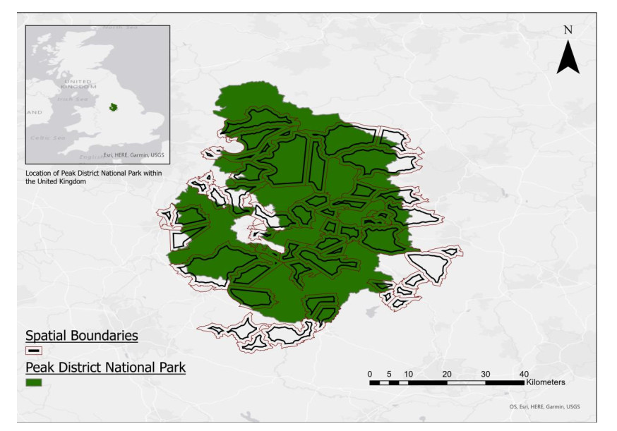
Protected Areas (PAs) are widely used to conserve biodiversity by protecting and restoring ecosystems while also contributing to socio-economic priorities. An increasing number of studies aim to examine the social impacts of PAs on aspects of people's well-being, such as, quality of life, livelihoods, and connectedness to nature. Despite the increase in literature on this topic, there are still few studies that explore possible robust methodological approaches to capturing and assessing the spatial distribution of impacts in a PA. This study aims to contribute to this research gap by comparing Bayesian spatial regression models that explore links between perceived social impacts and the relative location of local residents and communities in a PA. We use primary data collected from 227 individuals, via structured questionnaires, living in or near the Peak District National Park, United Kingdom. By comparing different models we were able to show that the location of respondents influences their perception of social impacts and that neighboring communities within the national park can have similar perceptions regarding social impacts. Simulation based on existing data using the Bootstrap sub-sampling was also conducted to validate the association between social impacts and mutual proximity of residents. Our findings suggest that this type of data is better treated, in terms of accounting for potential spatial effects, using models that allow for proximity effects to be stronger between people living nearby, e.g. between neighbors in the same community and have minimum effects otherwise. Understanding the spatial clustering of perceived social impacts in and around PA, is key to understanding their causes and to managing and mitigating them. Our findings highlight therefore the need to develop new methodological approaches to assessing and predicting accurately the spatial distribution of social impacts when designating PAs. The findings in this paper will assist practitioners in this regard by proposing approaches to the consideration of the distribution of social impacts when designing the boundaries of PAs alongside typical ecological and socio-economic criteria.
Citation: Chrysovalantis Malesios, Nikoleta Jones, Alfie Begley, James McGinlay. Methodological approaches to exploring the spatial variation in social impacts of protected areas: An intercomparison of Bayesian regression modeling approaches and potential implications[J]. Mathematical Biosciences and Engineering, 2024, 21(3): 3816-3837. doi: 10.3934/mbe.2024170
Protected Areas (PAs) are widely used to conserve biodiversity by protecting and restoring ecosystems while also contributing to socio-economic priorities. An increasing number of studies aim to examine the social impacts of PAs on aspects of people's well-being, such as, quality of life, livelihoods, and connectedness to nature. Despite the increase in literature on this topic, there are still few studies that explore possible robust methodological approaches to capturing and assessing the spatial distribution of impacts in a PA. This study aims to contribute to this research gap by comparing Bayesian spatial regression models that explore links between perceived social impacts and the relative location of local residents and communities in a PA. We use primary data collected from 227 individuals, via structured questionnaires, living in or near the Peak District National Park, United Kingdom. By comparing different models we were able to show that the location of respondents influences their perception of social impacts and that neighboring communities within the national park can have similar perceptions regarding social impacts. Simulation based on existing data using the Bootstrap sub-sampling was also conducted to validate the association between social impacts and mutual proximity of residents. Our findings suggest that this type of data is better treated, in terms of accounting for potential spatial effects, using models that allow for proximity effects to be stronger between people living nearby, e.g. between neighbors in the same community and have minimum effects otherwise. Understanding the spatial clustering of perceived social impacts in and around PA, is key to understanding their causes and to managing and mitigating them. Our findings highlight therefore the need to develop new methodological approaches to assessing and predicting accurately the spatial distribution of social impacts when designating PAs. The findings in this paper will assist practitioners in this regard by proposing approaches to the consideration of the distribution of social impacts when designing the boundaries of PAs alongside typical ecological and socio-economic criteria.

| [1] | Convention on Biological Diversity: Report of the expert workshop on the monitoring framework for the post-2020 global biodiversity framework, 2022. Available from: https://www.cbd.int/doc/c/3190/c3f4/1d9fe2d2dedc8c8b97023750/id-om-2022-01-02-en.pdf. |
| [2] | J. Day, N. Dudley, M. Hockings, G. Holmes, D. A. Laffoley, S. Stolton, et al., Guidelines for applying the IUCN Protected Area Management Categories to Marine Protected Areas, IUCN, Switzerland, 2012. |
| [3] |
S. Hernandez, M. D. Barnes, S. Duce, V. M. Adams, The impact of strictly protected areas in a deforestation hotspot. Conserv. Sci. Pract., 3 (2021), e479. https://doi.org/10.1111/csp2.479 doi: 10.1111/csp2.479

|
| [4] |
F. Romagosa, Physical health in green spaces: Visitors' perceptions and activities in protected areas around Barcelone, J. Outdoor Recreation Tourism, 23 (2018), 26–32. https://doi.org/10.1016/j.jort.2018.07.002 doi: 10.1016/j.jort.2018.07.002
|
| [5] |
D. Burdon, T. Potts, E. McKinley, S. Lew, R. Shilland, K. Gormley, et al., Expanding the role of participatory mapping to assess ecosystem service provision in local coastal environments. Ecosyst. Serv., 39 (2019), 101009. https://doi.org/10.1016/j.ecoser.2019.101009 doi: 10.1016/j.ecoser.2019.101009
|
| [6] |
G. J. Rodrigues, S. Villasante, I. S. Pinto, Non-material nature's contributions to people from a marine protected area support multiple dimensions of human well-being. Sustainab. Sci., 17 (2022), 793–808. https://doi.org/10.1007/s11625-021-01021-x doi: 10.1007/s11625-021-01021-x
|
| [7] |
N. Jones, Using perceived impacts, governance and social indicators to explain support for protected areas, Environ. Res. Lett., 18 (2023). https://doi.org/10.1088/1748-9326/acc95b doi: 10.1088/1748-9326/acc95b
|
| [8] |
J. McGinlay, N. Jones, C. Malesios, P. G. Dimitrakopoulos, A. Begley, S. Berzborn, et al., Exploring local public support for protected areas: What social factors influence stated and active support among local people?, Environ. Sci. Policy, 145 (2023), 250–261. https://doi.org/10.1016/j.envsci.2023.04.003 doi: 10.1016/j.envsci.2023.04.003
|
| [9] |
N. Jones, C. Malesios, A. Kantartzis, P. Dimitrakopoulos, The role of location and social impacts of protected areas on subjective wellbeing, Environ. Res. Lett., 15 (2020). https://doi.org/10.1088/1748-9326/abb96e doi: 10.1088/1748-9326/abb96e
|
| [10] |
S. J. Campbell, G. J. Edgar, R. D. Stuart-Smith, G. Soler, A. E. Bates, Fishing-gear restrictions and biomass gains for coral reef fishes in marine protected areas, Conserv. Biol., 32 (2017), 401–410. https://doi.org/10.1111/cobi.12996 doi: 10.1111/cobi.12996
|
| [11] |
J. S. Brandt, V. Butsic, B. Schwab, T. Kuemmerle, V. C. Radeloff, The relative effectiveness of protected areas, a logging ban and sacred areas for old growth forest protection in southwest China, Biol. Conserv., 181 (2015), 1–8. https://doi.org/10.1016/j.biocon.2014.09.043 doi: 10.1016/j.biocon.2014.09.043
|
| [12] |
N. J. Bennett, A. Di Franco, A. Calò, E. Nethery, F. Niccolini, M. Milazzo, et al., Local support for conservation is associated with perceptions of good governance, social impacts, and ecological effectiveness, Conserv. Lett., 12 (2019), e12640. https://doi.org/10.1111/conl.12640 doi: 10.1111/conl.12640
|
| [13] |
R. Naidoo, D. Gerkey, D. Hole, A. Pfaff, A. M. Ellis, C. D. Golden, et al., Evaluating the impacts of protected areas on human well-being across the developing world, Sci. Adv., 5 (2019), eaav3006. https://doi.org/10.1126/sciadv.aav3006 doi: 10.1126/sciadv.aav3006
|
| [14] |
J. McGinlay, J. Holtvoeth, A. Begley, J. Dörstel, A. Kockelmann, M. Lammertz, et al., Perceived social impacts of protected areas, their influence on local public support and their distribution across social groups: Evidence from the Eifel national park, Germany, during the COVID-19 pandemic, Sustainability, 15 (2023), 10848. https://doi.org/10.3390/su151410848. doi: 10.3390/su151410848
|
| [15] | A. D. Cliff, J. K. Ord, Spatial processes: models and applications, Taylor & Francis, 1981. |
| [16] | N. Jones, J. McGinlay, The impact of COVID-19 restrictions on local communities of Peak District National Park and management options during the Pandemic, 2021. Report available at: https://www.fidelio.landecon.cam.ac.uk/files/peak_district_report_final.pdf. |
| [17] |
J. A. Oldekop, G. Holmes, W. E. Harris, K. L. Evans, A global assessment of the social and conservation outcomes of protected areas, Conserv. Biol., 30 (2016), 133–141. https://doi.org/10.1111/cobi.12568 doi: 10.1111/cobi.12568
|
| [18] | N. Jones, J. McGinlay, V. Gkoumas, C. Malesios, V. Maguire-Rajpaul, L. Walker, SOCIAT: Social Impact Assessment Tool for Protected Areas, 2023. Available from: https://warwick.ac.uk/fac/arts/schoolforcross-facultystudies/research/projects/fidelio/sociat/about/. |
| [19] | B. Efron, The Jackknife, the Bootstrap and Other Resampling Plans, SIAM, Philadelphia, 1982. |
| [20] | B. Efron, D. Rogosa, R. Tibshirani, Resampling methods of estimation, in International Encyclopedia of the Social & Behavioral Sciences, Elsevier, New York, (2004), 13216–13220. |
| [21] | W. H. Greene, Models for Event Counts and Duration, Econometric Analysis, Upper Saddle River: Prentice Hall, (2008), 906–944. |
| [22] | P. McCullagh, J. Nelder, Generalized Linear Models, 2nd edition, Boca Raton: Chapman and Hall/CRC, 1989. |
| [23] |
F. Famoye, Restricted generalized Poisson regression model. Communications in statistics, Theory Methods, 22 (1991), 1335–1354. https://doi.org/10.1080/03610929308831089 doi: 10.1080/03610929308831089
|
| [24] |
C. Malesios, N. Demiris, K. Kalogeropoulos, I. Ntzoufras, Bayesian epidemic models for spatially aggregated count data, Stat. Med., 36 (2017), 3216–3230. https://doi.org/10.1002/sim.7364 doi: 10.1002/sim.7364
|
| [25] |
J. Besag, C. Kooperberg, Biometrika trust on conditional and intrinsic autoregression, Biometrika, 82 (1995), 733–746. https://doi.org/10.1093/biomet/82.4.733 doi: 10.1093/biomet/82.4.733
|
| [26] |
P. McCullagh, Regression models for ordinal data, J. Royal Stat. Soc. Series B, 42 (1980), 109–127. https://doi.org/10.1111/j.2517-6161.1980.tb01109.x doi: 10.1111/j.2517-6161.1980.tb01109.x
|
| [27] |
E. W. Duncan, N. M. White, K. Mengersen, Spatial smoothing in Bayesian models: a comparison of weights matrix specifications and their impact on inference, Int. J. Health Geographics, 16 (2017), 47. https://doi.org/10.1186/s12942-017-0120-x doi: 10.1186/s12942-017-0120-x
|
| [28] |
A. Getis, J. Aldstadt, Constructing the spatial weights matrix using a local statistic, Geographical Anal., 36 (2004), 90–104. https://doi.org/10.1111/j.1538-4632.2004.tb01127.x doi: 10.1111/j.1538-4632.2004.tb01127.x
|
| [29] |
P. Congdon, Random-effects models for migration attractivity and retentivity: a Bayesian methodology, J. Royal Stat. Soc. Series A, 173 (2010), 755–774. https://doi.org/10.1111/j.1467-985X.2009.00625.x doi: 10.1111/j.1467-985X.2009.00625.x
|
| [30] |
Z. Fric, V. Hula, M. Klimova, K. Zimmermann, M. Konvicka, Dispersal of four fritillary butterflies within identical landscape, Ecol. Res., 25 (2010), 543–552. https://doi.org/10.1007/s11284-009-0684-4 doi: 10.1007/s11284-009-0684-4
|
| [31] |
D. Obaromi, Spatial modelling of some conditional autoregressive priors in a disease mapping model the Bayesian approach, Biomed. J. Sci. Techn. Res., 14 (2019), 10681–10686. http://dx.doi.org/10.26717/BJSTR.2019.14.002555 doi: 10.26717/BJSTR.2019.14.002555
|
| [32] | H. Xia, B. P. Carlin, Spatio-temporal models with errors in covariates: mapping Ohio lung cancer mortality, Stat. Med., 17 (1998), 2025–2043. |
| [33] |
A. Earnest, G. Morgan, K. Mengersen, L. Ryan, R. Summerhayes, J. Beard, Evaluating the effect of neighbourhood weight matrices on smoothing properties of conditional autoregressive (CAR) models, Int. J. Health Geographics, 6 (2007), 1–12. https://doi.org/10.1186/1476-072x-6-54 doi: 10.1186/1476-072x-6-54
|
| [34] |
D. J. Lunn, A. Thomas, N. Best, D. Spiegelhalter, WinBUGS - A Bayesian modelling framework: Concepts, structure, and extensibility, Stat. Comput., 10 (2000), 325–337. https://doi.org/10.1023/A:1008929526011 doi: 10.1023/A:1008929526011
|
| [35] |
D. J. Spiegelhalter, N. G. Best, B. P. Carlin, A. Van Der Linde, Bayesian measures of model complexity and fit, J. Royal Stat. Soc. Series B, 64 (2002), 583–639. https://doi.org/10.1111/1467-9868.00353 doi: 10.1111/1467-9868.00353
|
| [36] |
S. E. Ahmed, A. Hussein, M. Al-Momani, Efficient estimation for the conditional autoregressive model, J. Stat. Comput. Simul., 85 (2015), 2569–2581. https://doi.org/10.1080/00949655.2014.893346 doi: 10.1080/00949655.2014.893346
|
| [37] |
C. Merow, M. J. Smith, T. C. Edwards Jr, A. Guisan, S. M. McMahon, S. Normand, et al., What do we gain from simplicity versus complexity in species distribution models?, Ecography, 37 (2014), 1267–1281. https://doi.org/10.1111/ecog.00845 doi: 10.1111/ecog.00845
|
| [38] |
M. Pogson, P. Smith, Effect of spatial data resolution on uncertainty, Environ. Model. Software, 63 (2015), 87–96. https://doi.org/10.1016/j.envsoft.2014.09.021 doi: 10.1016/j.envsoft.2014.09.021
|
| [39] |
J. O. Lloyd-Smith, Maximum likelihood estimation of the negative binomial dispersion parameter for highly overdispersed data, with applications to infectious diseases, PLoS ONE, 2 (2007), e180. https://doi.org/10.1371/journal.pone.0000180 doi: 10.1371/journal.pone.0000180
|
| [40] |
P. C. Consul, F. Famoye, Generalized poisson regression model, Commun. Stat. Theory Methods, 21 (1990), 89–109. https://doi.org/10.1080/03610929208830766 doi: 10.1080/03610929208830766
|
| [41] | D. Pennington, K. Gillen, P. Hill, Social Psychology, London: Hodder Education, (1999), 244–278. |
| [42] | K. Keizer, P. W. Schultz, Social norms and pro-environmental behaviour, in Environmental Psychology – An Introduction, (eds. L. Steg, A.E. Van den Berg and J.I.M. de Groot), Chichester: BPS Blackwell, (2013), 153–163. |


Figures(3) / Tables(7)

Chrysovalantis Malesios, Nikoleta Jones, Alfie Begley, James McGinlay. Methodological approaches to exploring the spatial variation in social impacts of protected areas: An intercomparison of Bayesian regression modeling approaches and potential implications[J]. Mathematical Biosciences and Engineering, 2024, 21(3): 3816-3837. doi: 10.3934/mbe.2024170


 DownLoad: