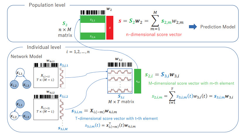
Brain functional connectivity is a useful biomarker for diagnosing brain disorders. Connectivity is measured using resting-state functional magnetic resonance imaging (rs-fMRI). Previous studies have used a sequential application of the graphical model for network estimation and machine learning to construct predictive formulas for determining outcomes (e.g., disease or health) from the estimated network. However, the resulting network had limited utility for diagnosis because it was estimated independent of the outcome. In this study, we proposed a regression method with scores from rs-fMRI based on supervised sparse hierarchical components analysis (SSHCA). SSHCA has a hierarchical structure that consists of a network model (block scores at the individual level) and a scoring model (super scores at the population level). A regression model, such as the multiple logistic regression model with super scores as the predictor, was used to estimate diagnostic probabilities. An advantage of the proposed method was that the outcome-related (supervised) network connections and multiple scores corresponding to the sub-network estimation were helpful for interpreting the results. Our results in the simulation study and application to real data show that it is possible to predict diseases with high accuracy using the constructed model.
Citation: Atsushi Kawaguchi. Network-based diagnostic probability estimation from resting-state functional magnetic resonance imaging[J]. Mathematical Biosciences and Engineering, 2023, 20(10): 17702-17725. doi: 10.3934/mbe.2023787
Brain functional connectivity is a useful biomarker for diagnosing brain disorders. Connectivity is measured using resting-state functional magnetic resonance imaging (rs-fMRI). Previous studies have used a sequential application of the graphical model for network estimation and machine learning to construct predictive formulas for determining outcomes (e.g., disease or health) from the estimated network. However, the resulting network had limited utility for diagnosis because it was estimated independent of the outcome. In this study, we proposed a regression method with scores from rs-fMRI based on supervised sparse hierarchical components analysis (SSHCA). SSHCA has a hierarchical structure that consists of a network model (block scores at the individual level) and a scoring model (super scores at the population level). A regression model, such as the multiple logistic regression model with super scores as the predictor, was used to estimate diagnostic probabilities. An advantage of the proposed method was that the outcome-related (supervised) network connections and multiple scores corresponding to the sub-network estimation were helpful for interpreting the results. Our results in the simulation study and application to real data show that it is possible to predict diseases with high accuracy using the constructed model.

| [1] |
S. Amemiya, H. Takao, O. Abe, Resting-State fMRI: Emerging Concepts for Future Clinical Application, J. Magn. Reson. Imaging, 2023 (2023). https://doi.org/10.1002/jmri.28894 doi: 10.1002/jmri.28894

|
| [2] | S. H. Joo, H. K. Lim, C. U. Lee, Three large-scale functional brain networks from resting-state functional MRI in subjects with different levels of cognitive impairment, Psychiatry Invest., 13 (2016). |
| [3] |
A. Chase, Altered functional connectivity in preclinical dementia, Nat. Rev. Neurol., 10 (2014), 11. https://doi.org/10.1038/nrneurol.2014.195 doi: 10.1038/nrneurol.2014.195
|
| [4] |
X. Chen, H. Zhang, Y. Gao, C. Y. Wee, G. Li, D. Shen, et al., High-order resting-state functional connectivity network for MCI classification, Human Brain Mapp., 37 (2016), 3282–3296. https://doi.org/10.1002/hbm.23240 doi: 10.1002/hbm.23240
|
| [5] |
B. Ibrahim, S. Suppiah, N. Ibrahim, M. Mohamad, H. Hassan, N. Nasser, et al., Diagnostic power of resting-state fMRI for detection of network connectivity in Alzheimer's disease and mild cognitive impairment: A systematic review, Human Brain Mapp., 42 (2021), 2941–2968. https://doi.org/10.1002/hbm.25369 doi: 10.1002/hbm.25369
|
| [6] |
S. L. Warren, A. A. Moustafa, Functional magnetic resonance imaging, deep learning, and Alzheimer's disease: A systematic review, J. Neuroimaging, 33 (2023), 5–18. https://doi.org/10.1111/jon.13063 doi: 10.1111/jon.13063
|
| [7] |
S. Khan, A. Gramfort, N. R. Shetty, M. G. Kitzbichler, S. Ganesan, J. M. Moran, et al., Local and long-range functional connectivity is reduced in concert in autism spectrum disorders, Proceed. Natl Acad. Sci., 110 (2013), 3107–3112. https://doi.org/10.1073/pnas.1214533110 doi: 10.1073/pnas.1214533110
|
| [8] |
H. Karbasforoushan, N. Woodward, Resting-state networks in schizophrenia, Curr. Top. Med. Chem., 12 (2012), 2404–2414. https://doi.org/10.2174/156802612805289863 doi: 10.2174/156802612805289863
|
| [9] | J. W. Murrough, C. G. Abdallah, A. Anticevic, K. A. Collins, P. Geha, L. A. Averill, et al., Reduced global functional connectivity of the medial prefrontal cortex in major depressive disorder, Human Brain Mapp., 37 (2016), 3214–3223. |
| [10] |
Z. Li, R. Chen, M. Guan, E. Wang, T. Qian, C. Zhao, et al., Disrupted brain network topology in chronic insomnia disorder: a resting-state fMRI study, NeuroImage Clin., 18 (2018), 178–185. https://doi.org/10.1016/j.nicl.2018.01.012 doi: 10.1016/j.nicl.2018.01.012
|
| [11] |
M. Brown, G. S. Sidhu, R. Greiner, N. Asgarian, M. Bastani, P. H. Silverstone, et al., ADHD-200 Global Competition: diagnosing ADHD using personal characteristic data can outperform resting state fMRI measurements, Front. Syst. Neurosci., 6 (2012), 69. https://doi.org/10.3389/fnsys.2012.00069 doi: 10.3389/fnsys.2012.00069
|
| [12] |
M. D. Rosenberg, E. S. Finn, D. Scheinost, X. Papademetris, X. Shen, R. T. Constable, et al., A neuromarker of sustained attention from whole-brain functional connectivity, Nat. Neurosci., 19 (2016), 165–171. https://doi.org/10.1038/nn.4179 doi: 10.1038/nn.4179
|
| [13] |
M. Rosenberg, E. Finn, D. Scheinost, R. Constable, M. Chun, Characterizing attention with predictive network models, Trends Cognit. Sci., 21 (2017), 290–302. https://doi.org/10.1016/j.tics.2017.01.011 doi: 10.1016/j.tics.2017.01.011
|
| [14] |
E. Finn, X. Shen, D. Scheinost, M. Rosenberg, J. Huang, M. Chun, et al., Functional connectome fingerprinting: identifying individuals using patterns of brain connectivity, Nat. Neurosci., 18 (2015), 1664–1671. https://doi.org/10.1038/nn.4135 doi: 10.1038/nn.4135
|
| [15] |
X. Shen, E. S. Finn, D. Scheinost, M. D. Rosenberg, M. M. Chun, X. Papademetris, et al., Using connectome-based predictive modeling to predict individual behavior from brain connectivity, Nat. Protoc., 12 (2017), 506–518. https://doi.org/10.1038/nprot.2016.178 doi: 10.1038/nprot.2016.178
|
| [16] |
P. H. Luckett, J. J. Lee, K. Y. Park, R. V. Raut, K. L. Meeker, E. M. Gordon, et al., Resting state network mapping in individuals using deep learning, Front. Neurol., 13 (2023), 1055437. https://doi.org/10.3389/fneur.2022.1055437 doi: 10.3389/fneur.2022.1055437
|
| [17] | J. Gao, J. Liu, Y. Xu, D. Peng, Z. Wang, Brain age prediction using graph neural network based on resting-state functional MRI in Alzheimer's disease, Front. Neurosci., 17 (Year), 1222751. |
| [18] |
H. I. Suk, C. Y. Wee, S. W. Lee, D. Shen, State-space model with deep learning for functional dynamics estimation in resting-state fMRI, NeuroImage, 129 (2016), 292–307. https://doi.org/10.1016/j.neuroimage.2016.01.005 doi: 10.1016/j.neuroimage.2016.01.005
|
| [19] |
H. Du, M. Xia, K. Zhao, X. Liao, H. Yang, Y. Wang, et al., PAGANI Toolkit: Parallel graph-theoretical analysis package for brain network big data, Human Brain Mapp., 39 (2018), 1869. https://doi.org/10.1002/hbm.23996 doi: 10.1002/hbm.23996
|
| [20] |
J. Liu, Y. Pan, F. X. Wu, J. Wang, Enhancing the feature representation of multi-modal MRI data by combining multi-view information for MCI classification, Neurocomputing, 400 (2020), 322–332. https://doi.org/10.1016/j.neucom.2020.03.006 doi: 10.1016/j.neucom.2020.03.006
|
| [21] |
C. Y. Wee, P. T. Yap, K. Denny, J. N. Browndyke, G. G. Potter, K. A. Welsh-Bohmer, et al., Resting-state multi-spectrum functional connectivity networks for identification of MCI patients, PloS One, 7 (2012), e37828. https://doi.org/10.1371/journal.pone.0037828 doi: 10.1371/journal.pone.0037828
|
| [22] |
B. Jie, D. Zhang, W. Gao, Q. Wang, C. Wee, D. Shen, Integration of network topological and connectivity properties for neuroimaging classification, IEEE Trans. Biomed. Eng., 61 (2013), 576–589. https://doi.org/10.1109/TBME.2013.2284195 doi: 10.1109/TBME.2013.2284195
|
| [23] |
X. Liang, J. Wang, C. Yan, N. Shu, K. Xu, G. Gong, et al., Effects of different correlation metrics and preprocessing factors on small-world brain functional networks: a resting-state functional MRI study, PloS One, 7 (2012), e32766. https://doi.org/10.1371/journal.pone.0032766 doi: 10.1371/journal.pone.0032766
|
| [24] |
Y. Wang, J. Kang, P. B. Kemmer, Y. Guo, An efficient and reliable statistical method for estimating functional connectivity in large scale brain networks using partial correlation, Front. Neurosci., 10 (2016), 123. https://doi.org/10.3389/fnins.2016.00123 doi: 10.3389/fnins.2016.00123
|
| [25] |
Y. Li, Y. Wang, G. Wu, F. Shi, L. Zhou, W. Lin, et al., Discriminant analysis of longitudinal cortical thickness changes in Alzheimer's disease using dynamic and network features, Neurobiol. Aging, 33 (2012), e15–e30. https://doi.org/10.1016/j.neurobiolaging.2010.11.008 doi: 10.1016/j.neurobiolaging.2010.11.008
|
| [26] |
C. Y. Wee, P. T. Yap, D. Zhang, L. Wang, D. Shen, Group-constrained sparse fMRI connectivity modeling for mild cognitive impairment identification, Brain Struct. Funct., 219 (2014), 641–656. https://doi.org/10.1007/s00429-013-0524-8 doi: 10.1007/s00429-013-0524-8
|
| [27] |
M. J. Rosa, L. Portugal, T. Hahn, A. J. Fallgatter, M. I. Garrido, J. Shawe-Taylor, et al., Sparse network-based models for patient classification using fMRI, Neuroimage, 105 (2015), 493–506. https://doi.org/10.1016/j.neuroimage.2014.11.021 doi: 10.1016/j.neuroimage.2014.11.021
|
| [28] |
J. Friedman, T. Hastie, R. Tibshirani, Sparse inverse covariance estimation with the graphical lasso, Biostatistics, 9 (2008), 432–441. https://doi.org/10.1093/biostatistics/kxm045 doi: 10.1093/biostatistics/kxm045
|
| [29] |
A. Kawaguchi, F. Yamashita, Supervised multiblock sparse multivariable analysis with application to multimodal brain imaging genetics, Biostatistics, 18 (2017), 651–665. https://doi.org/10.1093/biostatistics/kxx011 doi: 10.1093/biostatistics/kxx011
|
| [30] | A. Kawaguchi, Multivariate Analysis for Neuroimaging Data, CRC Press, (2021). https://doi.org/10.1201/9780429289606 |
| [31] |
N. Chaari, H. C. Akdağ, I. Rekik, Comparative survey of multigraph integration methods for holistic brain connectivity mapping, Med. Image Anal., 2023 (2023), 102741. https://doi.org/10.1016/j.media.2023.102741 doi: 10.1016/j.media.2023.102741
|
| [32] | A. Kawaguchi, R. Yamanaka, Gene expression signature-based prognostic risk score with network structure, Primary Central Nerv. Syst. Lymphoma, 2016 (2016), 67–80. |
| [33] |
H. Yoshida, A. Kawaguchi, F. Yamashita, K. Tsuruya, The utility of a network–based clustering method for dimension reduction of imaging and non-imaging biomarkers predictive of Alzheimer's disease, Sci. Rep., 8 (2018), 1–10. https://doi.org/10.1038/s41598-018-21118-1 doi: 10.1038/s41598-018-21118-1
|
| [34] | Y. Wang, L. Li, J. J. Li, H. Huang, Network Modeling in Biology: Statistical Methods for Gene and Brain Networks, Stat. Sci., 36 (2021), |
| [35] |
H. Shen, J. Z. Huang, Sparse principal component analysis via regularized low rank matrix approximation, J. Multivar. Anal., 99 (2008), 1015–1034. https://doi.org/10.1016/j.jmva.2007.06.007 doi: 10.1016/j.jmva.2007.06.007
|
Figures(5) / Tables(6)

Atsushi Kawaguchi. Network-based diagnostic probability estimation from resting-state functional magnetic resonance imaging[J]. Mathematical Biosciences and Engineering, 2023, 20(10): 17702-17725. doi: 10.3934/mbe.2023787


 DownLoad: