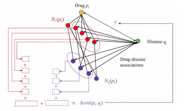
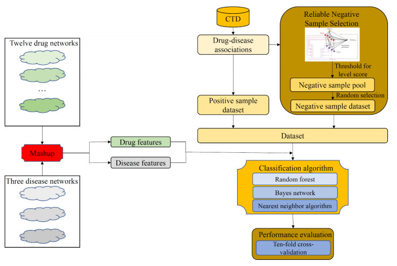
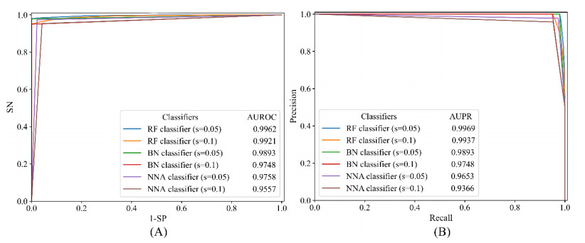
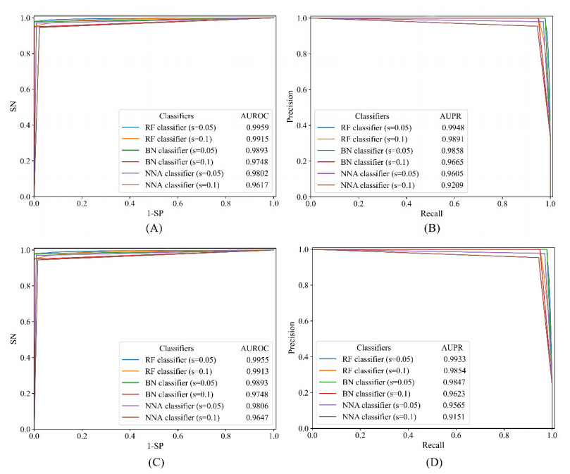
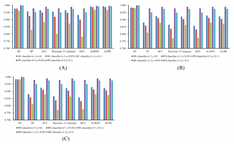
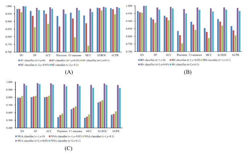
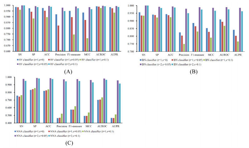
Drugs, which treat various diseases, are essential for human health. However, developing new drugs is quite laborious, time-consuming, and expensive. Although investments into drug development have greatly increased over the years, the number of drug approvals each year remain quite low. Drug repositioning is deemed an effective means to accelerate the procedures of drug development because it can discover novel effects of existing drugs. Numerous computational methods have been proposed in drug repositioning, some of which were designed as binary classifiers that can predict drug-disease associations (DDAs). The negative sample selection was a common defect of this method. In this study, a novel reliable negative sample selection scheme, named RNSS, is presented, which can screen out reliable pairs of drugs and diseases with low probabilities of being actual DDAs. This scheme considered information from k-neighbors of one drug in a drug network, including their associations to diseases and the drug. Then, a scoring system was set up to evaluate pairs of drugs and diseases. To test the utility of the RNSS, three classic classification algorithms (random forest, bayes network and nearest neighbor algorithm) were employed to build classifiers using negative samples selected by the RNSS. The cross-validation results suggested that such classifiers provided a nearly perfect performance and were significantly superior to those using some traditional and previous negative sample selection schemes.
Citation: Lei Chen, Kaiyu Chen, Bo Zhou. Inferring drug-disease associations by a deep analysis on drug and disease networks[J]. Mathematical Biosciences and Engineering, 2023, 20(8): 14136-14157. doi: 10.3934/mbe.2023632
Drugs, which treat various diseases, are essential for human health. However, developing new drugs is quite laborious, time-consuming, and expensive. Although investments into drug development have greatly increased over the years, the number of drug approvals each year remain quite low. Drug repositioning is deemed an effective means to accelerate the procedures of drug development because it can discover novel effects of existing drugs. Numerous computational methods have been proposed in drug repositioning, some of which were designed as binary classifiers that can predict drug-disease associations (DDAs). The negative sample selection was a common defect of this method. In this study, a novel reliable negative sample selection scheme, named RNSS, is presented, which can screen out reliable pairs of drugs and diseases with low probabilities of being actual DDAs. This scheme considered information from k-neighbors of one drug in a drug network, including their associations to diseases and the drug. Then, a scoring system was set up to evaluate pairs of drugs and diseases. To test the utility of the RNSS, three classic classification algorithms (random forest, bayes network and nearest neighbor algorithm) were employed to build classifiers using negative samples selected by the RNSS. The cross-validation results suggested that such classifiers provided a nearly perfect performance and were significantly superior to those using some traditional and previous negative sample selection schemes.

| [1] | D. McHale, M. Penny, Chapter 19 - Genomics, New drug development, and precision medicines, in Medical and Health Genomics, Oxford: Academic Press, (2016), 247-259. https://doi.org/10.1016/B978-0-12-420196-5.00019-8 |
| [2] |
C. W. Lindsley, New statistics on the cost of new drug development and the trouble with CNS drugs, ACS Chem. Neurosci., 5 (2014), 1142. https://doi.org/10.1021/cn500298z doi: 10.1021/cn500298z

|
| [3] |
M. R. Hurle, L. Yang, Q. Xie, D. K. Rajpal, P. Sanseau, P. Agarwal, Computational drug repositioning: from data to therapeutics, Clin. Pharmacol. Ther., 93 (2013), 335-341. https://doi.org/10.1038/clpt.2013.1 doi: 10.1038/clpt.2013.1
|
| [4] |
J. Li, S. Zheng, B. Chen, A. J. Butte, S. J. Swamidass, Z. Lu, A survey of current trends in computational drug repositioning, Briefings Bioinf., 17 (2016), 2-12. https://doi.org/10.1093/bib/bbv020 doi: 10.1093/bib/bbv020
|
| [5] |
Q. Dai, C. Bao, Y. Hai, S. Ma, T. Zhou, C. Wang, et al., MTGIpick allows robust identification of genomic islands from a single genome, Briefings Bioinf., 19 (2018), 361-373. https://doi.org/10.1093/bib/bbw118 doi: 10.1093/bib/bbw118
|
| [6] |
R. Kong, X. Xu, X. Liu, P. He, M. Q. Zhang, Q. Dai, 2SigFinder: the combined use of small-scale and large-scale statistical testing for genomic island detection from a single genome, BMC Bioinf., 21 (2020), 159. https://doi.org/10.1186/s12859-020-3501-2 doi: 10.1186/s12859-020-3501-2
|
| [7] |
D. Lai, L. Tan, X. Zuo, D. Liu, D. Jiao, G. Wan, et al., Prognostic ferroptosis-related lncRNA signatures associated with immunotherapy and chemotherapy responses in patients with stomach cancer, Front. Genet., 12 (2022), 798612. https://doi.org/10.3389/fgene.2021.798612 doi: 10.3389/fgene.2021.798612
|
| [8] |
F. Napolitano, Y. Zhao, V. M. Moreira, R. Tagliaferri, J. Kere, M. D'Amato, et al., Drug repositioning: a machine-learning approach through data integration, J. Cheminf., 5 (2013), 30. https://doi.org/10.1186/1758-2946-5-30 doi: 10.1186/1758-2946-5-30
|
| [9] | Z. Cui, Y. L. Gao, J. X. Liu, J. Wang, J. Shang, L. Y. Dai, The computational prediction of drug-disease interactions using the dual-network L2, 1-CMF method, BMC Bioinf., 20 (2019), 5. https://doi.org/10.1186/s12859-018-2575-6 |
| [10] | Y. Wang, S. Chen, N. Deng, Y. Wang, Drug repositioning by kernel-based integration of molecular structure, molecular activity, and phenotype data, PLoS One, 8 (2013), e78518. https://doi.org/10.1371/journal.pone.0078518 |
| [11] |
L. Lu, H. Yu, DR2DI: a powerful computational tool for predicting novel drug-disease associations, J. Comput.-Aided Mol. Des., 32 (2018), 633-642. https://doi.org/10.1007/s10822-018-0117-y doi: 10.1007/s10822-018-0117-y
|
| [12] |
C. Q. Gao, Y. K. Zhou, X. H. Xin, H. Min, P. F. Du, DDA-SKF: predicting drug-disease associations using similarity kernel fusion, Front. Pharmacol., 12 (2021), 784171. https://doi.org/10.3389/fphar.2021.784171 doi: 10.3389/fphar.2021.784171
|
| [13] |
G. Wu, J. Liu, C. Wang, Predicting drug-disease interactions by semi-supervised graph cut algorithm and three-layer data integration, BMC Med. Genomics, 10 (2017), 79. https://doi.org/10.1186/s12920-017-0311-0 doi: 10.1186/s12920-017-0311-0
|
| [14] |
A. P. Chiang, A. J. Butte, Systematic evaluation of drug-disease relationships to identify leads for novel drug uses, Clin. Pharmacol. Ther., 86 (2009), 507-510. https://doi.org/10.1038/clpt.2009.103 doi: 10.1038/clpt.2009.103
|
| [15] |
C. Wu, R. C. Gudivada, B. J. Aronow, A. G. Jegga, Computational drug repositioning through heterogeneous network clustering, BMC Syst. Biol., 7 (2013), S6. https://doi.org/10.1186/1752-0509-7-S5-S6 doi: 10.1186/1752-0509-7-S5-S6
|
| [16] |
H. Luo, J. Wang, M. Li, J. Luo, X. Peng, F. X. Wu, et al., Drug repositioning based on comprehensive similarity measures and Bi-Random walk algorithm, Bioinformatics, 32 (2016), 2664-2671. https://doi.org/10.1093/bioinformatics/btw228 doi: 10.1093/bioinformatics/btw228
|
| [17] |
W. Wang, S. Yang, X. Zhang, J. Li, Drug repositioning by integrating target information through a heterogeneous network model, Bioinformatics, 30 (2014), 2923-2930. https://doi.org/10.1093/bioinformatics/btu403 doi: 10.1093/bioinformatics/btu403
|
| [18] |
V. Martínez, C. Navarro, C. Cano, W. Fajardo, A. Blanco, DrugNet: network-based drug-disease prioritization by integrating heterogeneous data, Artif. Intell. Med., 63 (2015), 41-49. https://doi.org/10.1016/j.artmed.2014.11.003 doi: 10.1016/j.artmed.2014.11.003
|
| [19] | Y. F. Huang, H. Y. Yeh, V. W. Soo, Inferring drug-disease associations from integration of chemical, genomic and phenotype data using network propagation, BMC Med. Genomics, 6 (2013), S4. https://doi.org/10.1186/1755-8794-6-S3-S4 |
| [20] |
A. Gottlieb, G. Y. Stein, E. Ruppin, R. Sharan, PREDICT: a method for inferring novel drug indications with application to personalized medicine, Mol. Syst. Biol., 7 (2011), 496. https://doi.org/10.1038/msb.2011.26 doi: 10.1038/msb.2011.26
|
| [21] |
Y. Yang, L. Chen, Identification of drug-disease associations by using multiple drug and disease networks, Curr. Bioinf., 17 (2022), 48-59. https://doi.org/10.2174/1574893616666210825115406 doi: 10.2174/1574893616666210825115406
|
| [22] |
H. Jiang, Y. Huang, An effective drug-disease associations prediction model based on graphic representation learning over multi-biomolecular network, BMC Bioinf., 23 (2022), 9. https://doi.org/10.1186/s12859-021-04553-2 doi: 10.1186/s12859-021-04553-2
|
| [23] |
T. Kawichai, A. Suratanee, K. Plaimas, Meta-path based gene ontology profiles for predicting drug-disease associations, IEEE Access, 9 (2021), 41809-41820. https://doi.org/10.1109/ACCESS.2021.3065280 doi: 10.1109/ACCESS.2021.3065280
|
| [24] |
G. Fahimian, J. Zahiri, S. S. Arab, R. H. Sajedi, RepCOOL: computational drug repositioning via integrating heterogeneous biological networks, J. Transl. Med., 18 (2020), 375. https://doi.org/10.1186/s12967-020-02541-3 doi: 10.1186/s12967-020-02541-3
|
| [25] |
M. L. Zhang, B. W. Zhao, X. R. Su, Y. Z. He, Y. Yang, L. Hu, RLFDDA: a meta-path based graph representation learning model for drug-disease association prediction, BMC Bioinf., 23 (2022), 516. https://doi.org/10.1186/s12859-022-05069-z doi: 10.1186/s12859-022-05069-z
|
| [26] |
Z. Li, Q. Huang, X. Chen, Y. Wang, J. Li, Y. Xie, et al., Identification of drug-disease associations using information of molecular structures and clinical symptoms via deep convolutional neural network, Front. Chem., 7 (2019), 924. https://doi.org/10.3389/fchem.2019.00924 doi: 10.3389/fchem.2019.00924
|
| [27] |
Z. Wang, M. Zhou, C. Arnold, Toward heterogeneous information fusion: bipartite graph convolutional networks for in silico drug repurposing, Bioinformatics, 36 (2020), i525-i533. https://doi.org/10.1093/bioinformatics/btaa437 doi: 10.1093/bioinformatics/btaa437
|
| [28] |
B. W. Zhao, Z. H. You, L. Wong, P. Zhang, H. Y. Li, L. Wang, MGRL: predicting drug-disease associations based on multi-graph representation learning, Front. Genet., 12 (2021), 657182. https://doi.org/10.3389/fgene.2021.657182 doi: 10.3389/fgene.2021.657182
|
| [29] |
L. Breiman, Random forests, Mach. Learn., 45 (2001), 5-32. https://doi.org/10.1023/A:1010933404324 doi: 10.1023/A:1010933404324
|
| [30] |
T. Cover; P. Hart, Nearest neighbor pattern classification, IEEE Trans. Inf. Theory, 13 (1967), 21-27. https://doi.org/10.1109/TIT.1967.1053964 doi: 10.1109/TIT.1967.1053964
|
| [31] |
A. P. Davis, C. J. Grondin, R. J. Johnson, D. Sciaky, J. Wiegers, T. C. Wiegers, et al., Comparative toxicogenomics database (CTD): update 2021, Nucleic Acids Res., 49 (2021), D1138-D1143. https://doi.org/10.1093/nar/gkaa891 doi: 10.1093/nar/gkaa891
|
| [32] |
A. P. Davis, C. G. Murphy, R. Johnson, J. M. Lay, K. Lennon-Hopkins, C. Saraceni-Richards, et al., The comparative toxicogenomics database: update 2013, Nucleic Acids Res., 41 (2013), D1104-D1114. https://doi.org/10.1093/nar/gks994 doi: 10.1093/nar/gks994
|
| [33] | C. J. Mattingly, M. C. Rosenstein, G. T. Colby, J. N. Forrest, J. L. Boyer, The comparative toxicogenomics database (CTD): a resource for comparative toxicological studies, J. Exp. Zool. Part A: Comp. Exp. Biol., 305 (2006). https://doi.org/10.1002/jez.a.307 |
| [34] |
E. Sansone, F. G. De Natale, Z. H. Zhou, Efficient training for positive unlabeled learning, IEEE Trans. Pattern Anal. Mach. Intell., 41 (2018), 2584-2598. https://doi.org/10.1109/TPAMI.2018.2860995 doi: 10.1109/TPAMI.2018.2860995
|
| [35] |
D. Weininger, SMILES, a chemical language and information system. 1. Introduction to methodology and encoding rules, J. Chem. Inf. Comput. Sci., 28 (1988), 31-36. https://doi.org/10.1021/ci00057a005 doi: 10.1021/ci00057a005
|
| [36] |
X. Xiao, W. Zhu, B. Liao, J. Xu, C. Gu, B. Ji, et al., BPLLDA: predicting lncRNA-disease associations based on simple paths with limited lengths in a heterogeneous network, Front. Genet., 9 (2018), 411. https://doi.org/10.3389/fgene.2018.00411 doi: 10.3389/fgene.2018.00411
|
| [37] |
W. Ba-alawi, O. Soufan, M. Essack, P. Kalnis, V. B. Bajic, DASPfind: new efficient method to predict drug-target interactions, J. Cheminf., 8 (2016), 15. https://doi.org/10.1186/s13321-016-0128-4 doi: 10.1186/s13321-016-0128-4
|
| [38] |
Z. H. You, Z. A. Huang, Z. Zhu, G. Y. Yan, Z. W. Li, Z. Wen, et al., PBMDA: a novel and effective path-based computational model for miRNA-disease association prediction, PLoS Comput. Biol., 13 (2017), e1005455. https://doi.org/10.1371/journal.pcbi.1005455 doi: 10.1371/journal.pcbi.1005455
|
| [39] |
J. Gao, B. Hu, L. Chen, A path-based method for identification of protein phenotypic annotations, Curr. Bioinf., 16 (2021), 1214-1222. https://doi.org/10.2174/1574893616666210531100035 doi: 10.2174/1574893616666210531100035
|
| [40] |
M. Jiang, B. Zhou, L. Chen, Identification of drug side effects with a path-based method, Math. Biosci. Eng., 19 (2022), 5754-5771. https://doi.org/10.3934/mbe.2022269 doi: 10.3934/mbe.2022269
|
| [41] |
H. Ogata, S. Goto, K. Sato, W. Fujibuchi, H. Bono, M. Kanehisa, KEGG: Kyoto encyclopedia of genes and genomes, Nucleic Acids Res., 27 (1999), 29-34. https://doi.org/10.1093/nar/27.1.29 doi: 10.1093/nar/27.1.29
|
| [42] | M. Kanehisa, M. Furumichi, Y. Sato, M. Ishiguro-Watanabe, M. Tanabe, KEGG: integrating viruses and cellular organisms. Nucleic Acids Res., 49 (2021), D545-D551. https://doi.org/10.1093/nar/gkaa970 |
| [43] |
M. Kuhn, D. Szklarczyk, S. Pletscher-Frankild, T. H. Blicher, C. von Mering, L. J. Jensen, et al., STITCH 4: integration of protein–chemical interactions with user data, Nucleic Acids Res., 42 (2014), D401-D407. https://doi.org/10.1093/nar/gkt1207 doi: 10.1093/nar/gkt1207
|
| [44] |
D. S. Wishart, Y. D. Feunang, A. C. Guo, E. J. Lo, A. Marcu, J. R. Grant, et al., DrugBank 5.0: a major update to the DrugBank database for 2018, Nucleic Acids Res., 46 (2018), D1074-D1082. https://doi.org/10.1093/nar/gkx1037 doi: 10.1093/nar/gkx1037
|
| [45] |
M. Kuhn, M. Campillos, I. Letunic, L. J. Jensen, P. Bork, A side effect resource to capture phenotypic effects of drugs, Mol. Syst. Biol., 6 (2010), 343. https://doi.org/10.1038/msb.2009.98 doi: 10.1038/msb.2009.98
|
| [46] |
H. Cho, B. Berger, J. Peng, Compact integration of multi-network topology for functional analysis of genes, Cell Syst., 3 (2016), 540-548. https://doi.org/10.1016/j.cels.2016.10.017 doi: 10.1016/j.cels.2016.10.017
|
| [47] | H. Tong, C. Faloutsos, J. Pan, Fast random walk with restart and its applications, in Sixth International Conference on Data Mining (ICDM'06), (2006), 613-622. https://doi.org/10.1109/ICDM.2006.70 |
| [48] |
S. Kohler, S. Bauer, D. Horn, P. N. Robinson, Walking the interactome for prioritization of candidate disease genes, AJHG, 82 (2008), 949-958. https://doi.org/10.1016/j.ajhg.2008.02.013 doi: 10.1016/j.ajhg.2008.02.013
|
| [49] | R. Kohavi, A study of cross-validation and bootstrap for accuracy estimation and model selection, in Proceedings of the 14th international joint conference on Artificial intelligence, 2 (1995), 1137-1145. |
| [50] |
E. Frank, M. Hall, L. Trigg, G. Holmes, I. H. Witten, Data mining in bioinformatics using Weka, Bioinformatics, 20 (2004), 2479-2481. https://doi.org/10.1093/bioinformatics/bth261 doi: 10.1093/bioinformatics/bth261
|
| [51] | D. Powers, Evaluation: from precision, recall and f-measure to roc., informedness, markedness aand correlation, J. Mach. Learn. Technol., 2 (2011), 37-63. |
| [52] |
F. Huang, M. Fu, J. Li, L. Chen, K. Feng, T. Huang, et al., Analysis and prediction of protein stability based on interaction network, gene ontology, and KEGG pathway enrichment scores, Biochim. Biophys. Acta, Proteins Proteomics, 1871 (2023), 140889. https://doi.org/10.1016/j.bbapap.2023.140889 doi: 10.1016/j.bbapap.2023.140889
|
| [53] |
F. Huang, Q. Ma, J. Ren, J. Li, F. Wang, T. Huang, et al., Identification of smoking associated transcriptome aberration in blood with machine learning methods, Biomed Res. Int., 2023 (2023), 5333361. https://doi.org/10.1155/2023/5333361 doi: 10.1155/2023/5333361
|
| [54] |
M. Onesime, Z. Yang, Q. Dai, Genomic island prediction via Chi-Square test and random forest algorithm, Comput. Math. Methods Med., 2021 (2021), 9969751. https://doi.org/10.1155/2021/9969751 doi: 10.1155/2021/9969751
|
| [55] |
H. Wang, L. Chen, PMPTCE-HNEA: predicting metabolic pathway types of chemicals and enzymes with a heterogeneous network embedding algorithm, Curr. Bioinf., 2023 (2023). https://doi.org/10.2174/1574893618666230224121633 doi: 10.2174/1574893618666230224121633
|
| [56] |
C. Wu, L. Chen, A model with deep analysis on a large drug network for drug classification, Math. Biosci. Eng., 20 (2023), 383-401. https://doi.org/10.3934/mbe.2023018 doi: 10.3934/mbe.2023018
|
| [57] |
J. Ren, Y. Zhang, W. Guo, K. Feng, Y. Yuan, T. Huang, et al., Identification of genes associated with the impairment of olfactory and gustatory functions in COVID-19 via machine-learning methods, Life, 13 (2023), 798. https://doi.org/10.3390/life13030798 doi: 10.3390/life13030798
|
| [58] |
B. Matthews, Comparison of the predicted and observed secondary structure of T4 phage lysozyme, Biochim. Biophys. Acta, Protein Struct., 405 (1975), 442-451. https://doi.org/10.1016/0005-2795(75)90109-9 doi: 10.1016/0005-2795(75)90109-9
|
| [59] |
Z. Cheng, K. Huang, Y. Wang, H. Liu, J. Guan, S. Zhou, Selecting high-quality negative samples for effectively predicting protein-RNA interactions, BMC Syst. Biol., 11 (2017), 9. https://doi.org/10.1186/s12918-017-0390-8 doi: 10.1186/s12918-017-0390-8
|
| [60] |
X. Zhao, L. Chen, J. Lu, A similarity-based method for prediction of drug side effects with heterogeneous information, Math. Biosci., 306 (2018), 136-144. https://doi.org/10.1016/j.mbs.2018.09.010 doi: 10.1016/j.mbs.2018.09.010
|
| [61] |
Y. Jia, R. Zhao, L. Chen, Similarity-based machine learning model for predicting the metabolic pathways of compounds, IEEE Access, 8 (2020), 130687-130696. https://doi.org/10.1109/ACCESS.2020.3009439 doi: 10.1109/ACCESS.2020.3009439
|
| [62] |
S. Zhou, S. Wang, Q. Wu, R. Azim, W. Li, Predicting potential miRNA-disease associations by combining gradient boosting decision tree with logistic regression, Comput. Biol. Chem., 85 (2020), 107200. https://doi.org/10.1016/j.compbiolchem.2020.107200 doi: 10.1016/j.compbiolchem.2020.107200
|
| [63] |
Y. Zhao, X. Chen, J. Yin, Adaptive boosting-based computational model for predicting potential miRNA-disease associations, Bioinformatics, 35 (2019), 4730-4738. https://doi.org/10.1093/bioinformatics/btz297 doi: 10.1093/bioinformatics/btz297
|
| [64] |
F. Rayhan, S. Ahmed, S. Shatabda, D. M. Farid, Z. Mousavian, A. Dehzangi, et al., iDTI-ESBoost: identification of drug target interaction using evolutionary and structural features with boosting, Sci. Rep., 7 (2017), 17731. https://doi.org/10.1038/s41598-017-18025-2 doi: 10.1038/s41598-017-18025-2
|
| [65] |
H. Liang, L. Chen, X. Zhao, X. Zhang, Prediction of drug side effects with a refined negative sample selection strategy, Comput. Math. Methods Med., 2020 (2020), 1573543. https://doi.org/10.1155/2020/1573543 doi: 10.1155/2020/1573543
|
| [66] |
Z. Tian, Y. Yu, H. Fang, W. Xie, M. Guo, Predicting microbe–drug associations with structure-enhanced contrastive learning and self-paced negative sampling strategy, Briefings Bioinf., 24 (2023), bbac634. https://doi.org/10.1093/bib/bbac634 doi: 10.1093/bib/bbac634
|
Figures(7) / Tables(6)

Lei Chen, Kaiyu Chen, Bo Zhou. Inferring drug-disease associations by a deep analysis on drug and disease networks[J]. Mathematical Biosciences and Engineering, 2023, 20(8): 14136-14157. doi: 10.3934/mbe.2023632


 DownLoad: