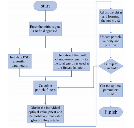
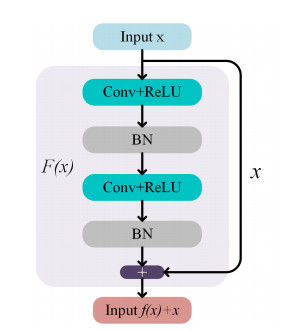
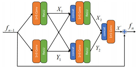
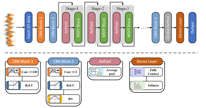
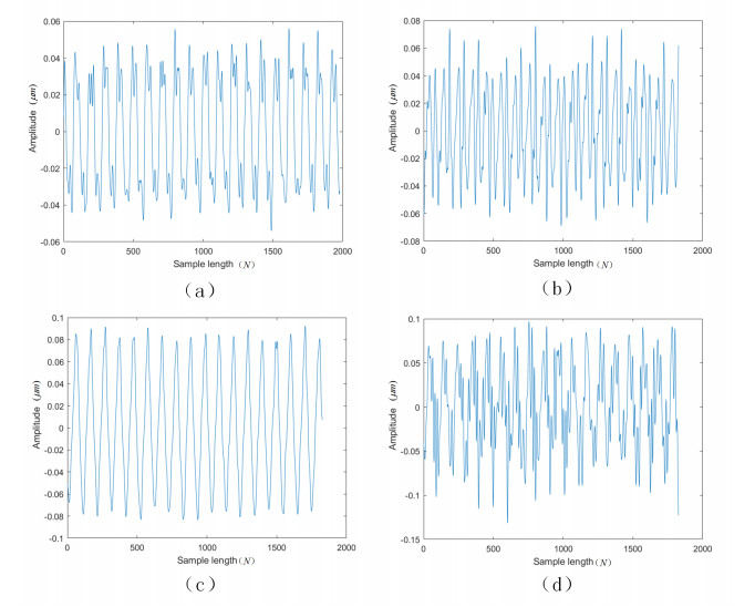
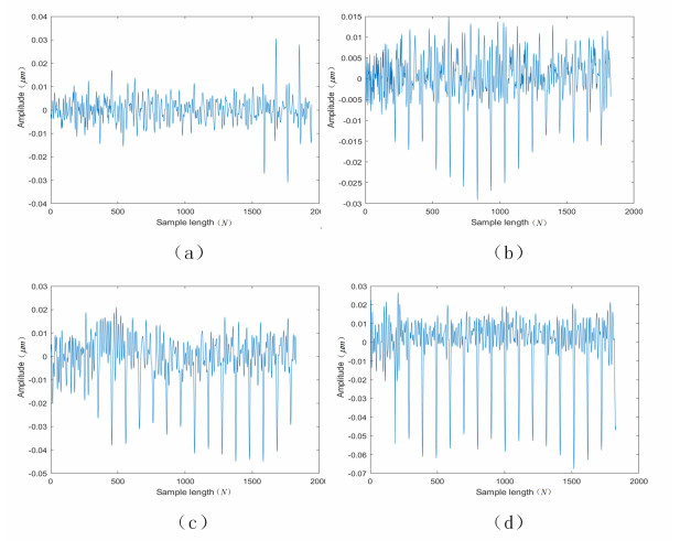
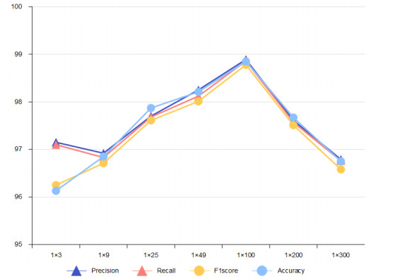
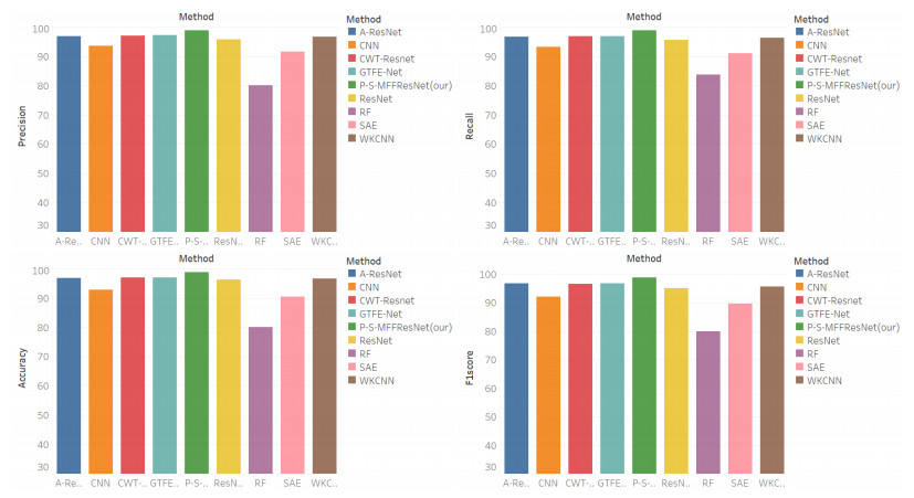
Due to the coupling effect of external environmental noise and vibration noise, the feature rate of the original hydroelectric unit fault signal is not prominent, which will affect the performance of fault diagnosis algorithms. To solve the above problems, this paper proposes a PSO-MCKD-MFFResnet algorithm for fault diagnosis of hydropower units (Particle swarm optimization, PSO; Maximum correlation kurtosis deconvolution, MCKD; Multi-scale feature fusion residual network, MFFResnet). In practical applications, the selection of key parameters in the traditional MCKD method is heavily dependent on prior knowledge. First, this paper proposes a PSO-MCKD enhancement algorithm for fault features, which uses the PSO algorithm to search for the influencing parameters of MCKD to enhance the features from the original fault signal. Second, a fault feature diagnosis algorithm based on MFFResnet is proposed to improve the utilization of local features. The multi-scale residual module is used to extract features at different scales and then put the enhanced signal into MFFResnet for training and classification. The experimental results show that our approach can accurately and effectively classify the fault types of hydropower units, with an accuracy rate of 98.85$ % $. It is superior to other representative algorithms in different indicators and has a good stability.
Citation: Xu Li, Zhuofei Xu, Yimin Wang. PSO-MCKD-MFFResnet based fault diagnosis algorithm for hydropower units[J]. Mathematical Biosciences and Engineering, 2023, 20(8): 14117-14135. doi: 10.3934/mbe.2023631
Due to the coupling effect of external environmental noise and vibration noise, the feature rate of the original hydroelectric unit fault signal is not prominent, which will affect the performance of fault diagnosis algorithms. To solve the above problems, this paper proposes a PSO-MCKD-MFFResnet algorithm for fault diagnosis of hydropower units (Particle swarm optimization, PSO; Maximum correlation kurtosis deconvolution, MCKD; Multi-scale feature fusion residual network, MFFResnet). In practical applications, the selection of key parameters in the traditional MCKD method is heavily dependent on prior knowledge. First, this paper proposes a PSO-MCKD enhancement algorithm for fault features, which uses the PSO algorithm to search for the influencing parameters of MCKD to enhance the features from the original fault signal. Second, a fault feature diagnosis algorithm based on MFFResnet is proposed to improve the utilization of local features. The multi-scale residual module is used to extract features at different scales and then put the enhanced signal into MFFResnet for training and classification. The experimental results show that our approach can accurately and effectively classify the fault types of hydropower units, with an accuracy rate of 98.85$ % $. It is superior to other representative algorithms in different indicators and has a good stability.

| [1] |
R. Santis, M. A. Costa, Extended isolation forests for fault detection in small hydroelectric plants, Sustainability, 12 (2020), 6421. https://doi.org/10.3390/su12166421 doi: 10.3390/su12166421

|
| [2] |
W. Liu, Y. Zheng, Z. Ma, B. Tian, Q. Chen, An intelligent fault diagnosis scheme for hydropower units based on the pattern recognition of axis orbits, Meas. Sci. Technol., 34 (2022). https://doi.org/10.1088/1361-6501/ac97ff doi: 10.1088/1361-6501/ac97ff
|
| [3] |
Y. Lei, B. Yang, X. Jiang, F. Jia, N. Li, A. K. Nandi, Applications of machine learning to machine fault diagnosis:a review and roadmap, Mech. Syst. Signal Process., 138 (2022), 106587. https://doi.org/10.1016/j.ymssp.2019.106587 doi: 10.1016/j.ymssp.2019.106587
|
| [4] |
K. Xu, Y. Li, C. Liu, X. Liu, X. Hao, J. Gao, Advanced data collection and analysis in data-driven manufacturing process, Chin. J. Mech. Eng., 33 (2020), 40–60. https://doi.org/10.1186/s10033-020-00459-x doi: 10.1186/s10033-020-00459-x
|
| [5] |
A. R. Al-Obaidi, Detection of cavitation phenomenon within a centrifugal Pump based on vibration analysis technique in both time and frequency domains, Exp. Tech., 44 (2020), 329–347. https://doi.org/10.1007/s40799-020-00362-z doi: 10.1007/s40799-020-00362-z
|
| [6] | J. Lin, C. Dou, Q. Wang, Comparisons of MFDFA, EMD and WT by neural network, mahalanobis distance and SVM in fault diagnosis of gearboxes, Sound Vib., 52 (2018), 11–15. |
| [7] | L. Bai, W. Xi, Early fault diagnosis of rolling bearing based empirical wavelet transform and spectral kurtosis, in 2018 IEEE International Conference on Prognostics and Health Management (ICPHM), (2018), 1–6. https://doi.org/10.1109/ICPHM.2018.8448997 |
| [8] |
J. S. Cheng, D. Yu, J. Tang, Y. Yang, Application of SVM and SVD technique based on EMD to the fault diagnosis of the rotating machinery, Shock Vib., 16 (2019), 89–98. https://doi.org/10.3233/SAV-2009-0457 doi: 10.3233/SAV-2009-0457
|
| [9] | Y. Hu, Q. Li, An adjustable envelope based EMD method for rollingbearing fault diagnosis, in IOP Conference Series: Materials Science and Engineering, 1043 (2021), 032017. https://doi.org/10.1088/1757-899X/1043/3/032017 |
| [10] |
Y. He, H. Wang, H. Xue, T. Zhang, Research on unknown fault diagnosis of rolling bearings based on parameter-adaptive maximum correlation kurtosis deconvolution, Rev. Sci. Instrum., 92 (2021), 055103. https://doi.org/10.1063/5.0046113 doi: 10.1063/5.0046113
|
| [11] |
Z. Li, A. Ming, W. Zhang, T. Liu, F. Chu, Y. Li, Fault feature extraction and enhancement of rolling element bearings based on maximum correlated kurtosis deconvolution and improved empirical wavelet transform, Appl. Sci., 9 (2019), 1876. https://doi.org/10.3390/app9091876 doi: 10.3390/app9091876
|
| [12] |
W. Hua, C. Luo, J. Leng, Z. Wang, Mine gearbox fault diagnosis based on multiwavelets and maximum correlated kurtosis deconvolution, J. Vibroeng., 19 (2017), 4185–4197. https://doi.org/10.21595/jve.2017.17497 doi: 10.21595/jve.2017.17497
|
| [13] |
F. Wang, C. Liu, W. Su, Z. Xue, Q. Han, H. Li, Combined failure diagnosis of slewing bearings based on MCKD-CEEMD-ApEn, Shock Vib., 2018 (2018), 1070–9622. https://doi.org/10.1155/2018/6321785 doi: 10.1155/2018/6321785
|
| [14] |
P. Wang, Y. Miao, Multi classification ERT flow pattern recognition method based on deep learning, J. Phys. Conf. Ser., 2181 (2022). https://doi.org/10.1088/1742-6596/2181/1/012010 doi: 10.1088/1742-6596/2181/1/012010
|
| [15] |
D. T. Hoang, H. J. Kang, A survey on deep learning based bearing fault diagnosis, Neurocomputing, 335 (2019), 327–335. https://doi.org/10.1016/j.neucom.2018.06.078 doi: 10.1016/j.neucom.2018.06.078
|
| [16] |
D. Yao, H. Liu, J. Yang, J. Zhang, Implementation of a novel algorithm of wheelset and axle box concurrent fault identification based on an efficient neural network with the attention mechanism, J. Intell. Manuf., 32 (2021), 0956–5515. https://doi.org/10.1007/s10845-020-01701-y doi: 10.1007/s10845-020-01701-y
|
| [17] |
B. Peng, Y. Bi, B. Xue, M. Zhang, S. Wan, A survey on fault diagnosis of rolling bearings, Algorithms, 15 (2022), 357. https://doi.org/10.3390/a15100347 doi: 10.3390/a15100347
|
| [18] |
H. Shao, H. Jiang, X. Li, T. Liang, Rolling bearing fault detection using continuous deep belief network with locally linear embedding, Comput. Ind., 96 (2018), 27–39. https://doi.org/10.1016/j.compind.2018.01.005 doi: 10.1016/j.compind.2018.01.005
|
| [19] |
B. Liu, C. Liu, Y. Zhou, D. Wang, Y. Dun, An unsupervised chatter detection method based on AE and merging GMM and K-mean, Mech. Syst. Signal Process., 186 (2023), 109861. https://doi.org/10.1016/j.ymssp.2022.109861 doi: 10.1016/j.ymssp.2022.109861
|
| [20] |
B. Ma, W. Cai, Y. Han, G. Yu, A novel probability confidence CNN model and its application in mechanical fault diagnosis, IEEE Trans. Instrum. Meas., 70 (2021), 1–11. https://doi.org/10.1109/TIM.2021.3077965 doi: 10.1109/TIM.2021.3077965
|
| [21] |
M. Sun, H. Wang, P. Liu, S. Huang, P. Fan, A sparse stacked denoising autoencoder with optimized transfer learning applied to the fault diagnosis of rolling bearings, Measurement, 146 (2019), 305–314. https://doi.org/10.1016/j.measurement.2019.06.029 doi: 10.1016/j.measurement.2019.06.029
|
| [22] |
D. Hoang, H. Kang, Rolling element bearing fault diagnosis using convolutional neural network and vibration image, Cognit. Syst. Res., 53 (2019), 42–50. https://doi.org/10.1016/j.cogsys.2018.03.002 doi: 10.1016/j.cogsys.2018.03.002
|
| [23] |
G. Liao, W. Gao, G. Yang, M. Guo, Hydroelectric generating unit fault diagnosis using 1-D convolutional neural network and gated recurrent unit in small hydro, IEEE Sens. J., 19 (2019), 9352–9363. https://doi.org/10.1109/JSEN.2019.2926095 doi: 10.1109/JSEN.2019.2926095
|
| [24] |
X. Wang, D. Mao, X. Li, Bearing fault diagnosis based on vibro-acoustic data fusion and 1D-CNN network, Measurement, 173 (2021), 108518. https://doi.org/10.1016/j.measurement.2020.108518 doi: 10.1016/j.measurement.2020.108518
|
| [25] |
X. Song, Y. Cong, Y Song, Y. Chen, P. Liang, A bearing fault diagnosis model based on CNN with wide convolution kernels, J. Ambient Intell. Hum. Comput., 13 (2022), 4041–4056. https://doi.org/10.1007/s12652-021-03177-x doi: 10.1007/s12652-021-03177-x
|
| [26] |
L. Jia, T. W. S. Chow, Y. Yuan, GTFE-Net: A Gramian time frequency enhancement CNN for bearing fault diagnosis, Eng. Appl. Artif. Intell., 119 (2023), 105794. https://doi.org/10.1016/j.engappai.2022.105794 doi: 10.1016/j.engappai.2022.105794
|
| [27] |
N. Sakli, H. Ghabri, B. O. Soufiene, F. Almalki, H. Sakli, O. Ali, et al., Resnet-50 for 12-Lead electrocardiogram automated diagnosis, Comput. Intell. Neurosci., 2022 (2022), 1–16. https://doi.org/10.1155/2022/7617551 doi: 10.1155/2022/7617551
|
| [28] |
W. Zhang, X. Li, Q. Ding, Deep residual learning-based fault diagnosis method for rotating machinery, ISA Trans., 95 (2019), 295–305. https://doi.org/10.1016/j.isatra.2018.12.025 doi: 10.1016/j.isatra.2018.12.025
|
| [29] |
Y. Wang, J. Liang, X. Gu, D. Ling, H. Yu, Multi-scale attention mechanism residual neural network for fault diagnosis of rolling bearings, Proc. Inst. Mech. Eng., Part C: J. Mech. Eng. Sci., 236 (2022), 10615–10629. https://doi.org/10.1177/09544062221104598 doi: 10.1177/09544062221104598
|
| [30] |
Y. Jin, C. Qin, Y. Huang, C. Liu, Actual bearing compound fault diagnosis based on active learning and decoupling attentional residual network, Measurement, 173 (2021), 108500. https://doi.org/10.1016/j.measurement.2020.108500 doi: 10.1016/j.measurement.2020.108500
|
| [31] |
Y. Chen, D. Zhang, H. Ni, J. Cheng, H. R. Karimi, Multi-scale split dual calibration network with periodic information for interpretable fault diagnosis of rotating machinery, Eng. Appl. Artif. Intell., 123 (2023), 106181. https://doi.org/10.1016/j.engappai.2023.106181 doi: 10.1016/j.engappai.2023.106181
|
| [32] |
Y. Chen, D. Zhang, H. Zhang, Q. Wang, Dual-path mixed-domain residual threshold networks for bearing fault diagnosis, IEEE Trans. Ind. Electron., 69 (2022), 13462–13472. https://doi.org/10.1109/TIE.2022.3144572 doi: 10.1109/TIE.2022.3144572
|
| [33] |
Y. Chen, D. Zhang, K. Zhu, R. Yan, An adaptive activation transfer learning approach for fault diagnosis, IEEE/ASME Trans. Mechatron., 2023 (2023), 1–12. https://doi.org/10.1109/TMECH.2023.3243533 doi: 10.1109/TMECH.2023.3243533
|
| [34] |
N. H. Phong, A. Santos, B. Ribeiro, PSO-convolutional neural networks with heterogeneous learning rate, IEEE Access, 10 (2022), 89970–89988. https://doi.org/10.1016/10.1109/ACCESS.2022.3201142 doi: 10.1016/10.1109/ACCESS.2022.3201142
|
| [35] |
Z. Jiang, J. Zheng, H. Pan, Sigmoid-based refined composite multiscale fuzzy entropy and t-SNE based fault diagnosis approach for rolling bearing, Measurement, 129 (2018), 332–342. https://doi.org/10.1016/j.measurement.2018.07.045 doi: 10.1016/j.measurement.2018.07.045
|
| [36] |
J. Yu, C. Xiao, T. Hu, Y. Gao, Selective weighted multi-scale morphological filter for fault feature extraction of rolling bearings, ISA Trans., 132 (2022), 544–556. https://doi.org/10.1016/j.isatra.2022.06.003 doi: 10.1016/j.isatra.2022.06.003
|
| [37] |
X. Dong, G. Li, Y. Jia, K. Xu, Multiscale feature extraction from the perspective of graph for hob fault diagnosis using spectral graph wavelet transform combined with improved random forest, Measurement, 176 (2021), 109178. https://doi.org/10.1016/j.measurement.2021.109178 doi: 10.1016/j.measurement.2021.109178
|
| [38] |
W. Huang, J. Chen, Y. Yang, G. Guo, An improved deep convolutional neural network with multi-scale information for bearing fault diagnosis, Neurocomputing, 395 (2019), 77–92. https://doi.org/10.1016/j.neucom.2019.05.052 doi: 10.1016/j.neucom.2019.05.052
|
| [39] |
B. Zhao, X. Zhang, Z. Zhan, Q. Wu, Deep multi-scale adversarial network with attention:a novel domain adaptation method for intelligent fault diagnosis, J. Manuf. Syst., 59 (2021), 565–576. https://doi.org/10.1016/j.jmsy.2021.03.024 doi: 10.1016/j.jmsy.2021.03.024
|
| [40] |
R. Fezai, K. Dhibi, M. Mansouri, M. Trabelsi, M. Hajji, K. Bouzrara, et al., Effective random forest-based fault detection and diagnosis for wind energy conversion systems, IEEE Sens. J., 21 (2021), 6914–6921. https://doi.org/10.1109/JSEN.2020.3037237 doi: 10.1109/JSEN.2020.3037237
|
| [41] |
J. Xu, S. Liang, X. Ding, R. Yan, A zero-shot fault semantics learning model for compound fault diagnosis, Expert Syst. Appl., 221 (2023), 119642. https://doi.org/10.1016/j.eswa.2023.119642 doi: 10.1016/j.eswa.2023.119642
|
Figures(8) / Tables(7)

Xu Li, Zhuofei Xu, Yimin Wang. PSO-MCKD-MFFResnet based fault diagnosis algorithm for hydropower units[J]. Mathematical Biosciences and Engineering, 2023, 20(8): 14117-14135. doi: 10.3934/mbe.2023631


 DownLoad: