Intelligent crowd sensing pickpocketing group identification using remote sensing data for secure smart cities

Jing Zhang; Ting Fan; Ding Lang; Yuguang Xu; Hong-an Li; Xuewen Li; Jing Zhang; Ting Fan; Ding Lang; Yuguang Xu; Hong-an Li; Xuewen Li

doi:10.3934/mbe.2023613

Mathematical Biosciences and Engineering

2023, Volume 20, Issue 8: 13777-13797. doi: 10.3934/mbe.2023613

Previous Article Next Article

Research article Special Issues

Intelligent crowd sensing pickpocketing group identification using remote sensing data for secure smart cities

1.
College of Computer Science and Technology, Xi'an University of Science and Technology, Xi'an 710600, China
2.
College of Energy Enginnering, Xi'an University of Science and Technology, Xi'an 710600, China
3.
College of Safety Science and Engineering, Xi'an University of Science and Technology, Xi'an 710600, China

Received: 23 March 2023 Revised: 27 May 2023 Accepted: 05 June 2023 Published: 16 June 2023

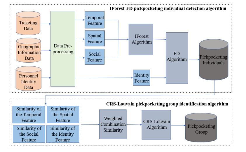
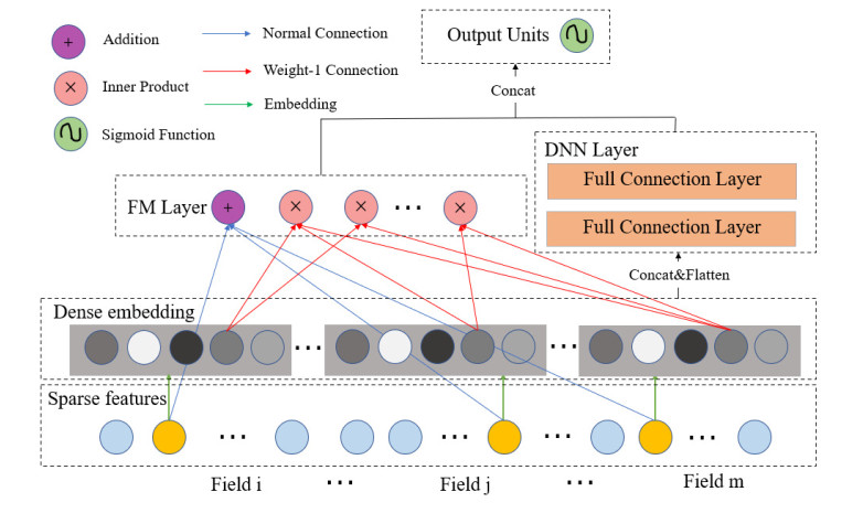
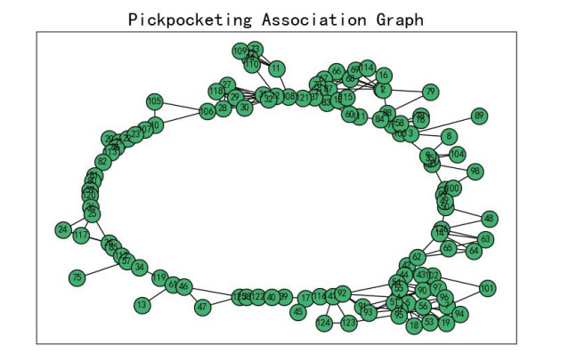
As a public infrastructure service, remote sensing data provided by smart cities will go deep into the safety field and realize the comprehensive improvement of urban management and services. However, it is challenging to detect criminal individuals with abnormal features from massive sensing data and identify groups composed of criminal individuals with similar behavioral characteristics. To address this issue, we study two research aspects: pickpocketing individual detection and pickpocketing group identification. First, we propose an IForest-FD pickpocketing individual detection algorithm. The IForest algorithm filters the abnormal individuals of each feature extracted from ticketing and geographic information data. Through the filtered results, the factorization machines (FM) and deep neural network (DNN) (FD) algorithm learns the combination relationship between low-order and high-order features to improve the accuracy of identifying pickpockets composed of factorization machines and deep neural networks. Second, we propose a community relationship strength (CRS)-Louvain pickpocketing group identification algorithm. Based on crowdsensing, we measure the similarity of temporal, spatial, social and identity features among pickpocketing individuals. We then use the weighted combination similarity as an edge weight to construct the pickpocketing association graph. Furthermore, the CRS-Louvain algorithm improves the modularity of the Louvain algorithm to overcome the limitation that small-scale communities cannot be identified. The experimental results indicate that the IForest-FD algorithm has better detection results in Precision, Recall and F1score than similar algorithms. In addition, the normalized mutual information results of the group division effect obtained by the CRS-Louvain pickpocketing group identification algorithm are better than those of other representative methods.
- crowdsensing,
- intelligent transportation,
- IForest-FD algorithm,
- CRS-Louvain algorithm
Citation: Jing Zhang, Ting Fan, Ding Lang, Yuguang Xu, Hong-an Li, Xuewen Li. Intelligent crowd sensing pickpocketing group identification using remote sensing data for secure smart cities[J]. Mathematical Biosciences and Engineering, 2023, 20(8): 13777-13797. doi: 10.3934/mbe.2023613

Related Papers:

Abstract

As a public infrastructure service, remote sensing data provided by smart cities will go deep into the safety field and realize the comprehensive improvement of urban management and services. However, it is challenging to detect criminal individuals with abnormal features from massive sensing data and identify groups composed of criminal individuals with similar behavioral characteristics. To address this issue, we study two research aspects: pickpocketing individual detection and pickpocketing group identification. First, we propose an IForest-FD pickpocketing individual detection algorithm. The IForest algorithm filters the abnormal individuals of each feature extracted from ticketing and geographic information data. Through the filtered results, the factorization machines (FM) and deep neural network (DNN) (FD) algorithm learns the combination relationship between low-order and high-order features to improve the accuracy of identifying pickpockets composed of factorization machines and deep neural networks. Second, we propose a community relationship strength (CRS)-Louvain pickpocketing group identification algorithm. Based on crowdsensing, we measure the similarity of temporal, spatial, social and identity features among pickpocketing individuals. We then use the weighted combination similarity as an edge weight to construct the pickpocketing association graph. Furthermore, the CRS-Louvain algorithm improves the modularity of the Louvain algorithm to overcome the limitation that small-scale communities cannot be identified. The experimental results indicate that the IForest-FD algorithm has better detection results in Precision, Recall and F1score than similar algorithms. In addition, the normalized mutual information results of the group division effect obtained by the CRS-Louvain pickpocketing group identification algorithm are better than those of other representative methods.

References

[1]	A. Falahati, E. Shafiee, Improve safety and security of intelligent railway transportation system based on balise using machine learning algorithm and fuzzy system, Int. J. Intell. Trans. Syst. Res., 20 (2021), 117–131. https://doi.org/10.1007/s13177-021-00274-1 doi: 10.1007/s13177-021-00274-1
[2]	K. Harshad, A Scalable, Reinforcement Learning Algorithm for Scheduling Railway Lines, IEEE Trans. Intell. Trans. Syst., 20 (2019), 727–736. https://doi.org/10.1109/TITS.2018.2829165 doi: 10.1109/TITS.2018.2829165
[3]	P. Dass, S. Misra, C. Roy, T-Safe: Trustworthy Service Provisioning for IoT-Based Intelligent Transport Systems, IEEE Trans. Veh. Technol., 69 (2020), 9509–9517. https://doi.org/10.1109/TVT.2020.3004047 doi: 10.1109/TVT.2020.3004047
[4]	J. Srinivas, A. K. Das, M. Wazid, A. V. Vasilakos, Designing Secure User Authentication Protocol for Big Data Collection in IoT-Based Intelligent Transportation System, IEEE Int. Things J., 8 (2021), 7727–7744. https://doi.org/10.1109/JIOT.2020.3040938 doi: 10.1109/JIOT.2020.3040938
[5]	C. Lin, G. J. Han, J. X. Du, T. T. Xu, L. Shu, Z. H. Lv, Spatiotemporal Congestion-Aware Path Planning Toward Intelligent Transportation Systems in Software-Defined Smart City IoT, IEEE Int. Things J., 7 (2020), 8012–8024. https://doi.org/10.1109/JIOT.2020.2994963 doi: 10.1109/JIOT.2020.2994963
[6]	S. Chavhan, D. Gupta, B. N. Chandana, A. Khanna, J. J. P. C. Rodrigues, IoT-Based Context-Aware Intelligent Public Transport System in a Metropolitan Area, IEEE Int. Things J., 7 (2020), 6023–6034. https://doi.org/10.1109/JIOT.2019.2955102 doi: 10.1109/JIOT.2019.2955102
[7]	Y. Liu, T. Feng, M. G. Peng, Z. B. Jiang, Z. Y. Xu, J. F. Guan, et al., COMP: Online Control Mechanism for Profit Maximization in Privacy-Preserving Crowdsensing, IEEE J. Select. Areas Commun., 38 (2020), 1614–1628. https://doi.org/10.1109/JSAC.2020.2999697 doi: 10.1109/JSAC.2020.2999697
[8]	C. Wang, Z. Y. Xie, L. Shao, Z. Z. Zhang, M. C. Zhou, Estimating travel speed of a road section through sparse crowdsensing data, IEEE Trans. Intell. Transp. Syst., 20 (2019), 3486–3495. https://doi.org/10.1109/TITS.2018.2877059 doi: 10.1109/TITS.2018.2877059
[9]	J. K. Ho, B. P. Jin, H. J. Young, Fuzzy filter for nonlinear sampled-data systems: Intelligent digital redesign approach, Int. J. Control Autom. Syst., 15 (2017), 603–610. https://doi.org/10.1007/s12555-015-0437-9 doi: 10.1007/s12555-015-0437-9
[10]	A. Capponi, C. Fiandrino, B. Kantarci, L. Foschini, D. Kliazovich, P. Bouvry, A survey on mobile crowdsensing systems: Challenges, solutions and opportunities, IEEE Commun. Surv. Tutor., 21 (2019), 2419–2465. https://doi.org/10.1109/COMST.2019.2914030 doi: 10.1109/COMST.2019.2914030
[11]	Z. Y. Zhou, J. H. Feng, B. Gu, B. Ai, S. Mumtaz, J. Rodriguez, et al., When mobile crowd sensing meets UAV: Energy-efficient task assignment and route planning, IEEE Trans. Commun., 66 (2018), 5526–5538. https://doi.org/10.1109/TCOMM.2018.2857461 doi: 10.1109/TCOMM.2018.2857461
[12]	K. K. Zhao, J. Zhang, L. F. Zhang, C. P. Li, H. Chen, CDSFM: A circular distributed SGLD-based factorization machines, Database Syst. Adv. Appl., 10828 (2018), 701–707. https://doi.org/10.1007/978-3-319-91458-9_43 doi: 10.1007/978-3-319-91458-9_43
[13]	M. Kahng, P. Y. Andrews, A. Kalro, D. H. Chau, ActiVis: Visual exploration of industry-scale deep neural network models, IEEE Trans. Vis. Comput. Graph., 24 (2018), 88–97. https://doi.org/10.1109/TVCG.2017.2744718 doi: 10.1109/TVCG.2017.2744718
[14]	N. Liu, X. L. Yu, L. Yao, X. J. Zhao, Mapping the cortical network arising from up-regulated amygdaloidal activation using Louvain algorithm, IEEE Trans. Neural Syst. Rehab. Eng., 26 (2018), 1169–1177. https://doi.org/10.1109/TNSRE.2018.2838075 doi: 10.1109/TNSRE.2018.2838075
[15]	S. Ramachandran, L. H. Palivela, C. Giridharan, An intelligent system to detect human suspicious activity using deep neural networks, J. Intell. Fuzzy Syst., 36 (2019), 4507–4518. http://dx.doi.org/10.3233/JIFS-179003 doi: 10.3233/JIFS-179003
[16]	D. Tsiktsiris, N. Dimitriou, A. Lalas, M. Dasygenis, K. Votis, D. Tzovaras, Real-time abnormal event detection for enhanced security in autonomous shuttles mobility infrastructures, Sensors, 20 (2020), 4943. https://doi.org/10.3390/s20174943 doi: 10.3390/s20174943
[17]	E. Selvi, M. Adimoolam, G. Karthi, K. Thinakaran, N. M. Balamurugan, R. Kannadasan, et al., Suspicious actions detection system using enhanced CNN and surveillance video, Electronics, 24 (2022), 4210. https://doi.org/10.3390/electronics11244210 doi: 10.3390/electronics11244210
[18]	D. Pascale, G. Cascavilla, M. Sangiovanni, D. Tamburri, W. J. Heuvel, Internet-of-things architectures for secure cyber–physical spaces: The VISOR experience report, J. Softw. Evol. Proc., 2022. https://doi.org/10.1002/smr.2511
[19]	P. Chen, J. Kurland, S. C. Shi, Predicting repeat offenders with machine learning: A case study of Beijing theives and burglars, in 2019 IEEE 4th International Conference on Big Data Analytics (ICBDA), (2019), 118–122. https://doi.org/10.1109/ICBDA.2019.8713192
[20]	B. Du, C. R. Liu, W. J. Zhou, Z. S. Hou, H. Xiong, Catch me if you can: Detecting pickpocket suspects from large-scale transit records, in Proceedings of the 22nd ACM SIGKDD International Conference on Knowledge Discovery and Data Mining, (2016), 87–96. https://doi.org/10.1145/2939672.2939687
[21]	A. Ogunleye, Q. G. Wang, XGBoost model for chronic kidney disease diagnosis, ACM Trans. Comput. Biol. Bioinform., 17 (2020), 2131–2140. https://doi.org/10.1109/TCBB.2019.2911071 doi: 10.1109/TCBB.2019.2911071
[22]	H. Gu, Y. Guo, H. Yang, P. Chen, M. Yao, J. Hou, Detecting pickpocketing offenders by analyzing Beijing metro subway data, in 2019 IEEE 4th International Conference on Big Data Analytics (ICBDA), (2019), 62–66. https://doi.org/10.1109/ICBDA.2019.8712833
[23]	S. A. Chun, V. A. Paturu, S. C Yuan, R. Pathak, V. Atluri, R. A. Nabil, Crime prediction model using deep neural networks, in Proceedings of the 20th Annual International Conference on Digital Government Research, (2019), 512–514. https://doi.org/10.1145/3325112.3328221
[24]	Z. H. Lu, X. F. Hu, L. F. Qiu, Analysis on hazard degree of cases of encroaching on property based on machine learning, J. Safe. Sci. Technol., 15 (2019), 29–35. 10.11731/j.issn.1673-193x.2019.12.005 doi: 10.11731/j.issn.1673-193x.2019.12.005
[25]	G. Xue, S. Liu, D. Gong, Identifying abnormal riding behavior in urban rail transit: A survey on "in-out" in the same subway station, IEEE Trans. Intell. Transp. Syst., 23 (2022), 3201–3213. https://doi.org/10.1109/TITS.2020.3032843 doi: 10.1109/TITS.2020.3032843
[26]	I.Pradhan, K.Potika, M.Eirinaki, P. Potikas, Exploratory data analysis and crime prediction for smart cities, in Proceedings of the 23rd International Database Applications & Engineering Symposium, 4 (2019), 1–9. https://doi.org/10.1145/3331076.3331114
[27]	S.W. Xu, J. N. Zhu, J. Z. Jiang, P. L. Shui, Sea-surface floating small target detection by multifeature detector based on isolation forest, IEEE J. Sel. Topics Appl. Earth Observ. Remote Sens., 14 (2021), 704–715. https://doi.org/10.1109/JSTARS.2020.3033063 doi: 10.1109/JSTARS.2020.3033063
[28]	F. S. Zhang, B. H. Jin, T. J. Ge, Q. Ji, Y. L. Cui, Who are my familiar strangers? Revealing hidden friend relations and common interests from smart card data, in Proceedings of the 25th ACM International on Conference on Information and Knowledge Management, (2016), 619–628. https://doi.org/10.1145/2983323.2983804
[29]	S. Liu, T. Yamamoto, E. Yao, T. Nakamura, Exploring travel pattern variability of public transport users through smart card data: Role of gender and age, IEEE Trans. Intell. Transp. Syst., 23 (2020), 4247–4256. https://doi.org/10.1109/TITS.2020.3043021 doi: 10.1109/TITS.2020.3043021
[30]	X. Zhao, Y. Zhang, Y. L. Hu, Z. S. Qian, H. Liu, B. C. Yin, Modeling relation proximity of passengers using public transit smart card data, in IEEE Intell. Transp. Syst. Mag., 14 (2020), 163–172. https://doi.org/10.1109/MITS.2019.2962145
[31]	J. Gravel, B. Allison, J. West-Fagan, M. McBride, G. E. Tita, Birds of a feather fight together: Status-enhancing violence, social distance and the emergence of homogenous gangs, J. Quant. Criminol., 34 (2018), 189–219. https://doi.org/10.1007/s10940-016-9331-8 doi: 10.1007/s10940-016-9331-8
[32]	L. Wang, Y. Zhang, X. Zhao, H. Liu, K. Zhang, Irregular travel groups detection based on cascade clustering in urban subway, IEEE Trans. Intell. Transp. Syst., 21 (2020), 2216–2225. https://doi.org/10.1109/TITS.2019.2933497 doi: 10.1109/TITS.2019.2933497
[33]	F. Troncoso, R. Weber, A novel approach to detect associations in criminal networks, Decis. Support Syst., 128 (2020), 113159. https://doi.org/10.1016/j.dss.2019.113159 doi: 10.1016/j.dss.2019.113159
[34]	M. Lim, A. Abdullah, N. Jhanjhi, M. K. Khan, Situation-aware deep reinforcement learning link prediction model for evolving criminal networks, IEEE Access, 8 (2020), 16550–16559. https://doi.org/10.1109/ACCESS.2019.2961805 doi: 10.1109/ACCESS.2019.2961805
[35]	C. Ma, Q. Lin, Y. Lin, X. Ma, Identification of multi-layer networks community by fusing nonnegative matrix factorization and topological structural information, Knowl.-Based Syst., 213 (2021), 1–14. https://doi.org/10.1016/j.knosys.2020.106666 doi: 10.1016/j.knosys.2020.106666
[36]	M. A. Tayebi, H. Y. Shahir, U. Glasser, P. L. Brantingham, Spatial patterns of offender groups, in 2018 IEEE International Conference on Intelligence and Security Informatics (ISI), (2018), 13–18. https://doi.org/10.1109/ISI.2018.8587365
[37]	X. Zhao, Y. Zhang, H. Liu, S. F. Wang, Z. Qian, Y. L. Hu, et al., Detecting pickpocketing gangs on buses with smart card data, IEEE Intell. Transp. Syst. Mag., 11 (2019), 181–199. https://doi.org/10.1109/MITS.2019.2919525 doi: 10.1109/MITS.2019.2919525
[38]	H. C. Qu, Z. L. Li, J. J. Wu, Integrated learning method for anomaly detection combining KLSH and isolation principles, in 2020 IEEE Congress on Evolutionary Computation (CEC), (2020), 1–6. https://doi.org/10.1109/CEC48606.2020.9185626
[39]	Z. Zhang, Z. Hu, H. Q. Yang, R. Zhu, D. C. Zuo, Factorization machines and deep views-based co-training for improving answer quality prediction in online health expert question-answering services, J. Biomed. Inf., 87 (2018), 21–36. https://doi.org/10.1016/j.jbi.2018.09.011 doi: 10.1016/j.jbi.2018.09.011
[40]	L. He, G. H. Wang, Z. Y. Hu, Learning depth from single images with deep neural network embedding focal length, IEEE Trans. Image Process., 27 (2018), 4676–4689. https://doi.org/10.1109/TIP.2018.2832296 doi: 10.1109/TIP.2018.2832296
[41]	J. Yang, G. Y. Wang, Q. H. Zhang, H. M. Wang, Knowledge distance measure for the multigranularity rough approximations of a fuzzy concept, IEEE Trans. Fuzzy Syst., 28 (2020), 706–717. https://doi.org/10.1109/TFUZZ.2019.2914622 doi: 10.1109/TFUZZ.2019.2914622
[42]	A. u. Rehman, A. Bermak, M. Hamdi, Shuffled frog-leaping and weighted cosine similarity for drift correction in gas sensors, IEEE Sensors J., 19 (2019), 12126–12136. https://doi.org/10.1109/JSEN.2019.2936602 doi: 10.1109/JSEN.2019.2936602
[43]	M. Besta, R. Kanakagiri, H. Mustafa, M. Karasikov, G. Rätsch, T. Hoefler, et al., Communication-efficient Jaccard similarity for high-performance distributed genome comparisons, in 2020 IEEE International Parallel and Distributed Processing Symposium (IPDPS), (2020), 1122–1132. https://doi.org/10.1109/IPDPS47924.2020.00118
[44]	G. Z. Li, A. N. Zhang, Q. Z. Zhang, D. Wu, C. J. Zhan, Pearson correlation coefficient-based performance enhancement of broad learning system for stock price prediction, IEEE Trans. Circuits Syst. II, 69 (2022), 2413–2417. https://doi.org/10.1109/TCSII.2022.3160266 doi: 10.1109/TCSII.2022.3160266
[45]	M. Seifikar, S. Farzi, M. Barati, C-Blondel: An efficient Louvain-based dynamic community detection algorithm, IEEE Trans. Comput. Social Syst., 7 (2020), 308–318. https://doi.org/10.1109/TCSS.2020.2964197 doi: 10.1109/TCSS.2020.2964197
[46]	M. Jiang, L. Song, Y. F. Wang, Z. Y. Li, H. B. Song, Fusion of the YOLOv4 network model and visual attention mechanism to detect low-quality young apples in a complex environment, Precis. Agric., 23 (2021), 559–577. https://doi.org/10.1007/s11119-021-09849-0 doi: 10.1007/s11119-021-09849-0
[47]	J. Cho, L. Schmalen, P. J. Winzer, Normalized generalized mutual information as a forward error correction threshold for probabilistically shaped QAM, in 2017 European Conference on Optical Communication (ECOC), (2017), 1–3. https://doi.org/10.1109/ECOC.2017.8345872

Reader Comments

Your name:*

Email:*
© 2023 the Author(s), licensee AIMS Press. This is an open access article distributed under the terms of the Creative Commons Attribution License (http://creativecommons.org/licenses/by/4.0)