Research on improved ant colony optimization for traveling salesman problem

Teng Fei; Xinxin Wu; Liyi Zhang; Yong Zhang; Lei Chen; Teng Fei; Xinxin Wu; Liyi Zhang; Yong Zhang; Lei Chen

doi:10.3934/mbe.2022381

Mathematical Biosciences and Engineering

2022, Volume 19, Issue 8: 8152-8186. doi: 10.3934/mbe.2022381

Previous Article Next Article

Research article

Research on improved ant colony optimization for traveling salesman problem

1.
Institute of Information Engineering, Tianjin University of Commerce, Tianjin 300134, China
2.
College of Science, Tianjin University of Commerce, Tianjin 300134, China

Received: 13 February 2022 Revised: 13 May 2022 Accepted: 24 May 2022 Published: 06 June 2022

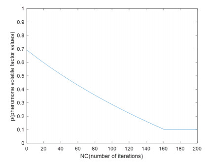
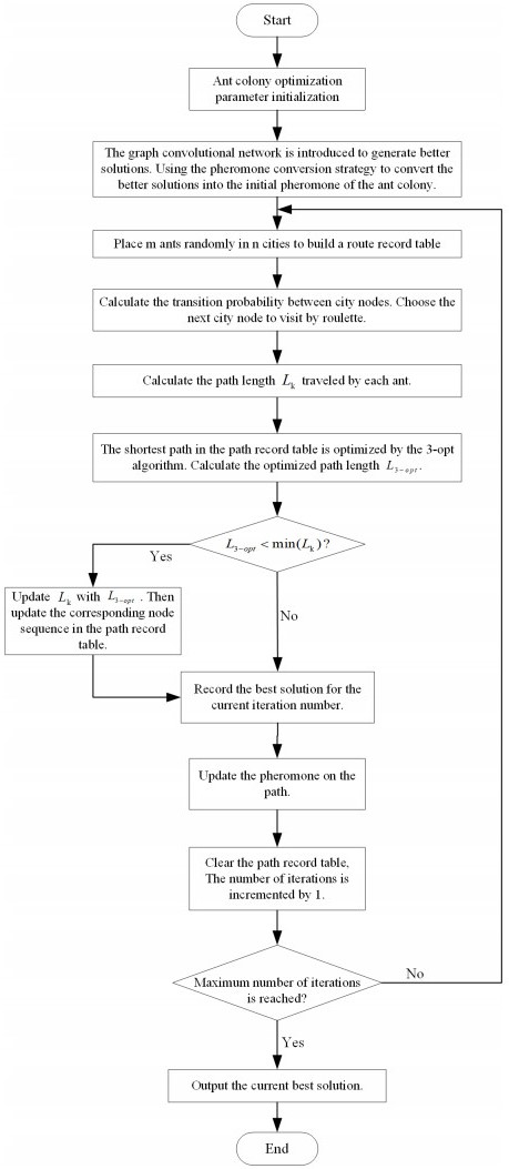
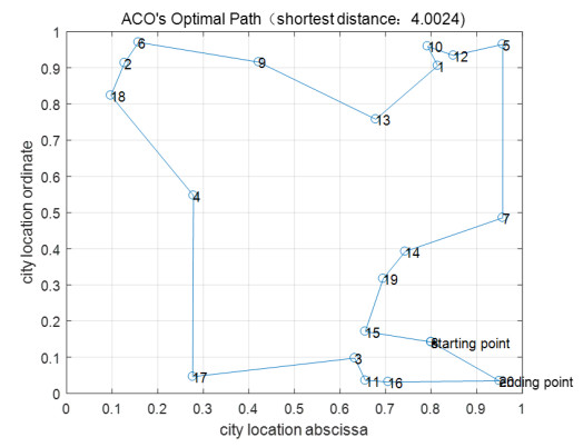
As one of the most popular combinatorial optimization problems, Traveling Salesman Problem (TSP) has attracted lots of attention from academia since it was proposed. Numerous meta-heuristics and heuristics have been proposed and used to solve the TSP. Although Ant Colony Optimization (ACO) is a natural TSP solving algorithm, in the process of solving it, there are also some shortcomings such as slow convergence speed and prone to fall into local optimum. Therefore, this paper proposes an improved ant colony optimization based on graph convolutional network: Graph Convolutional Network Improved Ant Colony Optimization (GCNIACO). The graph convolutional network is introduced to generate a better solution, and the better solution is converted into the pheromone on the initial path of the ACO. Thereby, the guiding effect of the pheromone concentration for the ants at the beginning of the algorithm is enhanced. In the meantime, through adaptive dynamic adjustment of the pheromone volatility factor and the introduction of the 3-opt algorithm, the algorithm's ability to jump out of the local optimum is enhanced. Finally, GCNIACO is simulated on TSP datasets and engineering application example. Comparing the optimization results with other classical algorithms, it is verified that the graph convolutional network improved ant colony optimization has better performance in obtaining the optimal solution.
- traveling salesman problem,
- ant colony optimization,
- graph convolutional network,
- dynamic pheromone volatility factor,
- 3-opt algorithm
Citation: Teng Fei, Xinxin Wu, Liyi Zhang, Yong Zhang, Lei Chen. Research on improved ant colony optimization for traveling salesman problem[J]. Mathematical Biosciences and Engineering, 2022, 19(8): 8152-8186. doi: 10.3934/mbe.2022381

Related Papers:

Abstract

As one of the most popular combinatorial optimization problems, Traveling Salesman Problem (TSP) has attracted lots of attention from academia since it was proposed. Numerous meta-heuristics and heuristics have been proposed and used to solve the TSP. Although Ant Colony Optimization (ACO) is a natural TSP solving algorithm, in the process of solving it, there are also some shortcomings such as slow convergence speed and prone to fall into local optimum. Therefore, this paper proposes an improved ant colony optimization based on graph convolutional network: Graph Convolutional Network Improved Ant Colony Optimization (GCNIACO). The graph convolutional network is introduced to generate a better solution, and the better solution is converted into the pheromone on the initial path of the ACO. Thereby, the guiding effect of the pheromone concentration for the ants at the beginning of the algorithm is enhanced. In the meantime, through adaptive dynamic adjustment of the pheromone volatility factor and the introduction of the 3-opt algorithm, the algorithm's ability to jump out of the local optimum is enhanced. Finally, GCNIACO is simulated on TSP datasets and engineering application example. Comparing the optimization results with other classical algorithms, it is verified that the graph convolutional network improved ant colony optimization has better performance in obtaining the optimal solution.

References

[1]	R. Laborda, Optimal combination of currency strategies, North Am. J. Econ. Finance, 43 (2018), 129–140. https://doi.org/10.1016/j.najef.2017.10.010 doi: 10.1016/j.najef.2017.10.010
[2]	S. Singh, K. C. Tiwari, Exploring the optimal combination of image fusion and classification techniques, Remote Sens. Appl.: Soc. Environ., 24 (2021), 100642. https://doi.org/10.1016/j.rsase.2021.100642 doi: 10.1016/j.rsase.2021.100642
[3]	J. H. Kim, I. Park, S. P. Chung, H. Y. Kim, I. K. Min, S. J. Kim, et al., Optimal combination of clinical examinations for neurologic prognostication of out-of-hospital cardiac arrest patients, Resuscitation, 155 (2020), 91–99. https://doi.org/10.1016/j.resuscitation.2020.07.014 doi: 10.1016/j.resuscitation.2020.07.014
[4]	X. L. Qin, Z. X. Liu, L. Tian, The optimal combination between selling mode and logistics service strategy in an e-commerce market, Eur. J. Oper. Res., 289 (2021), 639–651. https://doi.org/10.1016/j.ejor.2020.07.029 doi: 10.1016/j.ejor.2020.07.029
[5]	G. H. David, A. A. Antonio, E. Molina, A Combinatorial model to optimize air traffic flow management problems, Comput. Oper. Res., 112 (2019), 104768. https://doi.org/10.1016/j.cor.2019.104768 doi: 10.1016/j.cor.2019.104768
[6]	T. András, S. S. Maricruz, L. Végvári, G. P. Szijjártó, J. L. Margitfalvi, A. Trunschke, et al., Combinatorial optimization and synthesis of multiple promoted MoVNbTe catalysts for oxidation of propane to acrylic acid, Catal. Today, 363 (2021), 45–54. https://doi.org/10.1016/j.cattod.2019.03.047 doi: 10.1016/j.cattod.2019.03.047
[7]	S. Bharati, P. Podder, M. R. H. Mondal, Hybrid deep learning for detecting lung diseases from X-ray images, Inf. Med. Unlocked, 20 (2020), 100391. https://doi.org/10.1016/j.imu.2020.100391 doi: 10.1016/j.imu.2020.100391
[8]	G. Laporte, The traveling salesman problem: an overview of exact and approximate algorithms, Eur. J. Oper. Res., 59 (1992), 231–247. https://doi.org/10.1016/0377-2217(92)90138-Y doi: 10.1016/0377-2217(92)90138-Y
[9]	A. Colorni, M. Dorigo, V. Maniezzo, Distributed optimization by ant colonies, in Proceedings of the first European conference on artificial life, Elsevier Publishing, (1991), 134–142.
[10]	M. Gunduz, M. Aslan, DJAYA: A discrete Jaya algorithm for solving traveling salesman problem, Appl. Soft Comput., 105 (2021), 107275. https://doi.org/10.1016/j.asoc.2021.107275 doi: 10.1016/j.asoc.2021.107275
[11]	K. Panwar, K. Deep, Discrete Grey Wolf Optimizer for symmetric travelling salesman problem, Appl. Soft Comput., 105 (2021), 107298. https://doi.org/10.1016/j.asoc.2021.107298 doi: 10.1016/j.asoc.2021.107298
[12]	S. K. R. Kanna, K. Sivakumar, N. Lingaraj, Development of Deer Hunting linked Earthworm Optimization Algorithm for solving large scale Traveling Salesman Problem, Knowledge-Based Syst., 227 (2021), 107199. https://doi.org/10.1016/j.knosys.2021.107199 doi: 10.1016/j.knosys.2021.107199
[13]	M. M. Krishna, N. Panda, S. K. Majhi, Solving traveling salesman problem using hybridization of rider optimization and spotted hyena optimization algorithm, Expert Syst. Appl., 183 (2021), 115353. https://doi.org/10.1016/j.eswa.2021.115353 doi: 10.1016/j.eswa.2021.115353
[14]	Y. Saji, M. Barkatou, A discrete bat algorithm based on Lévy flights for Euclidean traveling salesman problem, Expert Syst. Appl., 172 (2021), 114639. https://doi.org/10.1016/j.eswa.2021.114639 doi: 10.1016/j.eswa.2021.114639
[15]	G. H. Al-Gaphari, R. Al-Amry, A. S. Al-Nuzaili, Discrete crow-inspired algorithms for traveling salesman problem, Eng. Appl. Artif. Intell., 97 (2021), 104006. https://doi.org/10.1016/j.engappai.2020.104006 doi: 10.1016/j.engappai.2020.104006
[16]	Y. Huang, X. N. Shen, X. You, A discrete shuffled frog-leaping algorithm based on heuristic information for traveling salesman problem, Appl. Soft Comput., 102 (2021), 107085. https://doi.org/10.1016/j.asoc.2021.107085 doi: 10.1016/j.asoc.2021.107085
[17]	I. M. Ali, D. Essam, K. Kasmarik, A novel design of differential evolution for solving discrete traveling salesman problems, Swarm Evol. Comput., 52 (2020), 100607. https://doi.org/10.1016/j.swevo.2019.100607 doi: 10.1016/j.swevo.2019.100607
[18]	M. A. H. Akhand, S. I. Ayon, S. A. Shahriyar, N. Siddique, H. Adeli, Discrete spider monkey optimization for travelling salesman problem, Appl. Soft Comput., 86 (2020), 105887. https://doi.org/10.1016/j.asoc.2019.105887 doi: 10.1016/j.asoc.2019.105887
[19]	M. Deudon, P. Cournut, A. Lacoste, Y. Adulyasak, L. M. Rousseau, Learning heuristics for the TSP by policy gradient, in Integration of Constraint Programming, Artificial Intelligence, and Operations Research, Springer, Cham, 10848 (2018), 170–181. https://doi.org/10.1007/978-3-319-93031-2_12
[20]	M. O. R. Prates, P. H. C. Avelar, H. Lemos, L. Lamb, M. Vardi, Learning to solve np-complete problems: A graph neural network for decision tsp, in Proceedings of the AAAI Conference on Artificial Intelligence, 33 (2019), 4731–4738.
[21]	W. Kool, H. V. Hoof, M. Welling, Attention, learn to solve routing problems!, preprint, arXiv: 1803.08475.
[22]	Y. J. Hu, Z. Zhang, Y. Yao, X. P. Huyan, X. S. Zhou, W. S. Lee, A bidirectional graph neural network for traveling salesman problems on arbitrary symmetric graphs, Eng. Appl. Artif. Intell., 97 (2021), 104061. https://doi.org/10.1016/j.engappai.2020.104061 doi: 10.1016/j.engappai.2020.104061
[23]	A. Ragmani, A. Elomri, N. Abghour, K. Moussaid, M. Rida, An improved hybrid fuzzy-ant colony algorithm applied to load balancing in cloud computing environment, Procedia Comput. Sci., 151 (2019), 519–526. https://doi.org/10.1016/j.procs.2019.04.070 doi: 10.1016/j.procs.2019.04.070
[24]	S. Ebadinezhad, DEACO: adopting dynamic evaporation strategy to enhance ACO algorithm for the traveling salesman problem, Eng. Appl. Artif. Intell., 92 (2020), 103649. https://doi.org/10.1016/j.engappai.2020.103649 doi: 10.1016/j.engappai.2020.103649
[25]	J. Li, Y. Xia, B. Li, Z. G. Zeng, A pseudo-dynamic search ant colony optimization algorithm with improved negative feedback mechanism, Cognit. Syst. Res., 62 (2020), 1–9. https://doi.org/10.1016/j.cogsys.2020.03.001 doi: 10.1016/j.cogsys.2020.03.001
[26]	A. F. Tuani, E. Keedwell, M. Collett, Heterogenous Adaptive Ant Colony Optimization with 3-opt local search for the Travelling Salesman Problem, Appl. Soft Comput., 97 (2020), 106720. https://doi.org/10.1016/j.asoc.2020.106720 doi: 10.1016/j.asoc.2020.106720
[27]	J. Y. Zheng, X. Q. Cheng, J. J. Fu, Application research of improved ant colony algorithm in TSP, Comput. Simul., 38 (2021), 126–130+167.
[28]	M. L. Li, Q. Z. Li, Path Planning of Unmanned Crane Based on Improved Ant Colony Algorithm, Comput. Simul., 38 (2021), 172–176+226.
[29]	X. H. Tang, S. J. Xin, Improved ant colony algorithm for mobile robot path planning, Comput. Eng. Appl., in press.
[30]	C. Liu, L. Wu, X. D. Huang, W. S. Xiao, Improved dynamic adaptive ant colony optimization algorithm to solve pipe routing design, Knowledge-Based Syst., 237 (2022), 107846. https://doi.org/10.1016/j.knosys.2021.107846 doi: 10.1016/j.knosys.2021.107846
[31]	L. W. Yang, L. X. Fu, N. Guo, Z. Yang, H. Q. Guo, X. Y. Xu, Path planning with multi-factor improved ant colony algorithm, Comput. Integr. Manuf. Syst., in press.
[32]	M. L. He, Z. X. Wei, X. H. Wu, Y. T. Peng, An improved ant colony optimization algorithm for vehicle routing problem with soft time windows, Comput. Integr. Manuf. Syst., in press.
[33]	S. B. Wang, R. Hu, B. Qian, M. Y. Liu, Improved Ant Colony Optimization for Solving Green Periodic Vehicle Routing Problem, Control Eng. China, in press. https://doi.org/10.14107/j.cnki.kzgc.20200581
[34]	A. C. Cinar, S. Korkmaz, M. S. Kiran, A discrete tree-seed algorithm for solving symmetric traveling salesman problem, Eng. Sci. Technol. Int. J., 23 (2020), 879–890. https://doi.org/10.1016/j.jestch.2019.11.005 doi: 10.1016/j.jestch.2019.11.005
[35]	G. Campuzano, C. Obreque, M. M. Aguayo, Accelerating the Miller–Tucker–Zemlin model for the asymmetric traveling salesman problem, Expert Syst. Appl., 148 (2020), 113229. https://doi.org/10.1016/j.eswa.2020.113229 doi: 10.1016/j.eswa.2020.113229
[36]	H. P. Hipólito, S. G. Juan-José, A Branch-and-cut algorithm for the split-demand one-commodity pickup-and-delivery travelling salesman problem, Eur. J. Oper. Res., 297 (2022), 467–483. https://doi.org/10.1016/j.ejor.2021.05.040 doi: 10.1016/j.ejor.2021.05.040
[37]	O. Cheikhrouhou, I. Khoufi, A comprehensive survey on the multiple traveling salesman problem: Applications, approaches and taxonomy, Comput. Sci. Rev., 40 (2021), 100369. https://doi.org/10.1016/j.cosrev.2021.100369 doi: 10.1016/j.cosrev.2021.100369
[38]	M. Cornu, T. Cazenave, D. Vanderpooten, Perturbed decomposition algorithm applied to the multi-objective traveling salesman problem, Comput. Oper. Res., 79 (2017), 314–330. https://doi.org/10.1016/j.cor.2016.04.025 doi: 10.1016/j.cor.2016.04.025
[39]	H. B. Duan, The Principle and Application of Ant Colony Algorithm, Science Press, Beijing, 2005.
[40]	L. Ma, G. Zhu, A. B. Ning, Ant Colony Optimization Algorithm, Science Press, Beijing, 2007.
[41]	J. W. Zhuo, B. W. Li, Y. S. Wei, J. Qin, Application of MATLAB in Mathematical Modeling, Beihang University Press, Beijing, 2014.
[42]	X. Bresson, T. Laurent, Residual gated graph convNets, preprint, arXiv: 1711.07553. https://doi.org/10.48550/arXiv.1711.07553
[43]	K. J. Chaitanya, T. Laurent, X. Bresson, An efficient graph convolutional network technique for the travelling salesman problem, preprint, arXiv: 1906.01227. https://doi.org/10.48550/arXiv.1906.01227
[44]	Z. Yang, H. Zhou, L. Q. Zhu, W. Li, Chemical reaction ant colony optimization algorithm, Appl. Res. Comput., 31 (2014), 2925–2927+2946.
[45]	X. H. Zhong, On the approximation ratio of the 3-Opt algorithm for the (1, 2)-TSP, Oper. Res. Lett., 49 (2021), 515–521. https://doi.org/10.1016/j.orl.2021.05.012 doi: 10.1016/j.orl.2021.05.012
[46]	D. L. Applegate, R. E. Bixby, V. Chvatal, W. J. Cook, The Traveling Salesman Problem: A Computational Study, Princeton university press, Princeton, 2006.
[47]	D. P. Kingma, J. Ba, Adam: A method for stochastic optimization, preprint, arXiv: 1412.6980. https://doi.org/10.48550/arXiv.1412.6980
[48]	Z. W. Ye, Z. B. Zheng, Configuration of Parameters $\alpha$, $\beta$, $\rho$, in ant algorithm, Geomatics Inf. Sci. Wuhan Univ., 29 (2004), 597–601.
[49]	T. R. Zhang, B. K. Wu, F. Q. Zhou, Research on improved ant colony algorithm for robot global path planning, Comput. Eng. Appl., 58 (2022), 282–291.
[50]	D. H. Wolpert, W. G. Macready, No free lunch theorems for optimization, IEEE Trans. Evol. Comput., 1 (1997), 67–82. https://doi.org/10.1109/4235.585893 doi: 10.1109/4235.585893
[51]	S. Bharati, P. Podder, M. R. H. Mondal, N. Gandhi, Optimized NASNet for Diagnosis of COVID-19 from Lung CT Images, Intell. Syst. Design Appl., 1351 (2021), 647–656. https://doi.org/10.1007/978-3-030-71187-0_59 doi: 10.1007/978-3-030-71187-0_59
[52]	TSPLIB, Available from: http://comopt.ifi.uni-heidelberg.de/software/TSPLIB95/tsp/.
[53]	S. W. Yu, MATLAB Optimization Algorithm Case Analysis and Application, Tsinghua University Press, Beijing, 2014.
[54]	L. Yu, F. Shi, H. Wang, F. Hu, 30 Case Studies of MATLAB Intelligent Algorithms, 2$^nd$ edition, Beijing University of Aeronautics and Astronautics Press, Beijing, 2015.
[55]	J. Derrac, S. García, D. Molina, F. Herrera, A practical tutorial on the use of nonparametric statistical tests as a methodology for comparing evolutionary and swarm intelligence algorithms, Swarm Evol. Comput., 1 (2011), 3–18. https://doi.org/10.1016/j.swevo.2011.02.002 doi: 10.1016/j.swevo.2011.02.002
[56]	A. Khamparia, S. Bharati, P. Podder, D. Gupta, A. Khanna, T. K. Phung, et al., Diagnosis of breast cancer based on modern mammography using hybrid transfer learning, Multidimension. Syst. Signal Process., 32 (2021), 747–765. https://doi.org/10.1007/s11045-020-00756-7 doi: 10.1007/s11045-020-00756-7
[57]	G. B. Dantzig, J. H. Ramser, The truck dispatching problem, Manage. Sci., 6 (1959), 80–91. https://doi.org/10.1287/mnsc.6.1.80 doi: 10.1287/mnsc.6.1.80
[58]	Z. F. Wang, H. L. Du, S. F. An, C. J. Zhang, An improved ant colony algorithm based on vehicle routing problem, J. Huaqiao Univ. (Nat. Sci.), 34 (2013), 36–39.
[59]	T. Fei, L. Y. Zhang, Y. S. Sun, Solution of vehicle routing optimization problem based on DNA-ant colony algorithm, Comput. Eng., 40 (2014), 206–213.

Reader Comments

Your name:*

Email:*
© 2022 the Author(s), licensee AIMS Press. This is an open access article distributed under the terms of the Creative Commons Attribution License (http://creativecommons.org/licenses/by/4.0)