Order batching and order picking with 3D positioning of the articles: solution through a hybrid evolutionary algorithm

Fabio M. Miguel; Mariano Frutos; Máximo Méndez; Fernando Tohmé; Fabio M. Miguel; Mariano Frutos; Máximo Méndez; Fernando Tohmé

doi:10.3934/mbe.2022259

Mathematical Biosciences and Engineering

2022, Volume 19, Issue 6: 5546-5563. doi: 10.3934/mbe.2022259

Previous Article Next Article

Research article Special Issues

Order batching and order picking with 3D positioning of the articles: solution through a hybrid evolutionary algorithm

1.
Universidad Nacional de Río Negro, Sede Alto Valle y Valle Medio, Argentina
2.
Engineering Department, Universidad Nacional del Sur, IIESS UNS CONICET, Argentina
3.
Universidad de Las Palmas de Gran Canaria (ULPGC), Instituto Universitario SIANI, Spain
4.
Economics Department, Universidad Nacional del Sur, INMABB UNS CONICET, Argentina

Academic Editor: Yang Kuang

Received: 29 December 2021 Revised: 02 March 2022 Accepted: 22 March 2022 Published: 28 March 2022

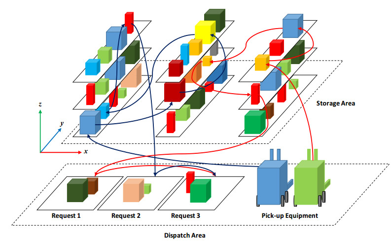
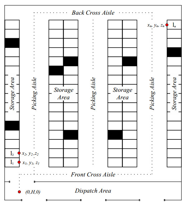
A critical factor in the logistic management of firms is the degree of efficiency of the operations in distribution centers. Of particular interest is the pick-up process, since it is the costliest operation, amounting to 50 and up to 75% of the total cost of the activities in storage facilities. In this paper we jointly address the order batching problem (OBP) and the order picking problem (OPP). The former problem amounts to find optimal batches of goods to be picked up, by restructuring incoming orders by either splitting up large orders or combining small orders into larger ones that can then be picked in a single picking tour. The OPP, in turn, involves identifying optimal sequences of visits to the storage positions in which the goods to be included in each batch are stored. We seek to design a plan that minimizes the total operational cost of the pick-up process, proportional to the displacement times around the storage area as well as to all the time spent in pick-ups and finishing up orders to be punctually delivered. Earliness or tardiness will induce inefficiency costs, be it because of the excessive use of space or breaches of contracts with customers. Tsai, Liou and Huang in 2008 have generated 2D and 3D instances. In previous works we have addressed the 2D ones, achieving very good results. Here we focus on 3D instances (the articles are placed at different levels in the storage center), which involve a higher complexity. This contributes to improve the performance of the hybrid evolutionary algorithm (HEA) applied in our previous works.
- order batching,
- order picking,
- evolutionary algorithm,
- local search,
- optimization
Citation: Fabio M. Miguel, Mariano Frutos, Máximo Méndez, Fernando Tohmé. Order batching and order picking with 3D positioning of the articles: solution through a hybrid evolutionary algorithm[J]. Mathematical Biosciences and Engineering, 2022, 19(6): 5546-5563. doi: 10.3934/mbe.2022259

Related Papers:

Abstract

A critical factor in the logistic management of firms is the degree of efficiency of the operations in distribution centers. Of particular interest is the pick-up process, since it is the costliest operation, amounting to 50 and up to 75% of the total cost of the activities in storage facilities. In this paper we jointly address the order batching problem (OBP) and the order picking problem (OPP). The former problem amounts to find optimal batches of goods to be picked up, by restructuring incoming orders by either splitting up large orders or combining small orders into larger ones that can then be picked in a single picking tour. The OPP, in turn, involves identifying optimal sequences of visits to the storage positions in which the goods to be included in each batch are stored. We seek to design a plan that minimizes the total operational cost of the pick-up process, proportional to the displacement times around the storage area as well as to all the time spent in pick-ups and finishing up orders to be punctually delivered. Earliness or tardiness will induce inefficiency costs, be it because of the excessive use of space or breaches of contracts with customers. Tsai, Liou and Huang in 2008 have generated 2D and 3D instances. In previous works we have addressed the 2D ones, achieving very good results. Here we focus on 3D instances (the articles are placed at different levels in the storage center), which involve a higher complexity. This contributes to improve the performance of the hybrid evolutionary algorithm (HEA) applied in our previous works.

References

[1]	E. Sancaklı, İ. Dumlupınar, A. O. Akçın, E. Çınar, İ. Geylani, Z. Düzgit, Design of a routing algorithm for efficient order picking in a non-traditional rectangular warehouse layout, in Digitizing Production Systems (eds. N. M. Durakbasa, M. G. Gençyılmaz), LNME, (2022), 401–412. https://doi.org/10.1007/978-3-030-90421-0_33
[2]	C. Y. Tsai, J. J. Liou, T. M. Huang, Using a multiple-GA method to solve the batch picking problem: considering travel distance and order due time. Int. J. Prod. Res., 46 (2008), 6533–6555. https://doi.org/10.1080/00207540701441947 doi: 10.1080/00207540701441947
[3]	F. Miguel, M. Frutos, F. Tohmé, D. A. Rossit, A memetic algorithm for the integral OBP/OPP problem in a logistics distribution center, Uncertain Supply Chain Manage., 7 (2019), 203–214. https://doi.org/10.5267/j.uscm.2018.10.005 doi: 10.5267/j.uscm.2018.10.005
[4]	F. Miguel, M. Frutos, M. Méndez, F. Tohmé, Solving order batching / picking problems with an evolutionary algorithm, in Communications in Computer and Information Science (eds. D. A. Rossit, F. Tohmé, G. Mejía Delgadillo), (2021), 177–186. https://doi.org/10.1007/978-3-030-76307-7_14
[5]	T. Van Gils, K. Ramaekers, K. Braekers, B. Depaire, A. Carisa, Increasing order picking efficiency by integrating storage, batching, zone picking, and routing policy decisions, Int. J. Prod. Econo., 197 (2018), 243–261. https://doi.org/10.1016/j.ijpe.2017.11.021 doi: 10.1016/j.ijpe.2017.11.021
[6]	R. De Koster, E. S. Van der Poort, M. Wolters, Efficient order batching methods in warehouses, Int. J. Prod. Res., 37 (1999), 1479–1504. https://doi.org/10.1080/002075499191094 doi: 10.1080/002075499191094
[7]	R. De Koster, T. Le-Duc, K. J. Roodbergen, Design and control of warehouse order picking: A literature review, Eur. J. Oper. Res., 182 (2007), 481–501. https://doi.org/10.1016/j.ejor.2006.07.009 doi: 10.1016/j.ejor.2006.07.009
[8]	F. M. Hofmann, S. E. Visagie, The effect of order batching on a cyclical order picking system, in Computational Logistics ICCL 2021 (eds. M. Mes, E. Lalla Ruiz, S. Voß), LNCS, 13004 (2021), 252–268. https://doi.org/10.1007/978-3-030-87672-2_17
[9]	G. Villarreal-Zapata, T. E. Salais-Fierro, J. A. Saucedo-Martínez, Intelligent system for selection of order picking technologies, Wireless Networks, 26 (2020), 1–8. https://doi.org/10.1007/s11276-020-02262-x doi: 10.1007/s11276-020-02262-x
[10]	E. Tappia, D. Roy, M. Melacini, R. De Koster, Integrated storage-order picking systems: technology, performance models, and design insights, Eur. J. Oper., 274 (2018), 947–965. https://doi.org/10.1016/j.ejor.2018.10.048 doi: 10.1016/j.ejor.2018.10.048
[11]	Ö. Öztürkoğlu, D. Hoser, A discrete cross aisle design model for order-picking warehouses, Eur. J. Oper. Res., 275 (2018), 411–430. https://doi.org/10.1016/j.ejor.2018.11.037 doi: 10.1016/j.ejor.2018.11.037
[12]	E. H. Grosse, C. H. Glock, The effect of worker learning on manual order picking processes, Int. J. Prod. Econo., 170 (2015), 882–890. https://doi.org/10.1016/j.ijpe.2014.12.018 doi: 10.1016/j.ijpe.2014.12.018
[13]	I. Žulj, C. H. Glock, E. H. Grosse, M. Schneider, Picker routing and storage-assignment strategies for precedence-constrained order picking, Comput. Ind. Eng., 123 (2018), 338–347. https://doi.org/10.1016/j.cie.2018.06.015 doi: 10.1016/j.cie.2018.06.015
[14]	M. C. Chen, H. P. Wu, An association-based clustering approach to order batching considering customer demand patterns, Omega, 33 (2005), 333–343. https://doi.org/10.1016/J.OMEGA.2004.05.003 doi: 10.1016/J.OMEGA.2004.05.003
[15]	S. Henn, S. Y. Koch, G. Wäscher, Order batching in order picking warehouses: a survey of solution approaches, in Warehousing in the Global Supply Chain (eds. R. Manzini), Springer, (2012), 105–137. https://doi.org/10.1007/978-1-4471-2274-6_6
[16]	S. Henn, G. Wäscher, Tabu search heuristics for the order batching problem in manual order picking systems, Eur. J. Oper. Res., 222 (2012), 484–494. https://doi.org/10.1016/j.ejor.2012.05.049 doi: 10.1016/j.ejor.2012.05.049
[17]	K. Rana, Order-picking in narrow-aisle warehouse, Int. J. Phys. Distrib. Logistics, 20 (1991), 9–15. https://doi.org/10.1108/09600039010005133 doi: 10.1108/09600039010005133
[18]	H. Hwang, D. Kim, Order-batching heuristics based on cluster analysis in a low-level picker-to-part warehousing system, Eur. J. Oper. Res., 43 (2005), 3657–3670. https://doi.org/10.1080/00207540500151325 doi: 10.1080/00207540500151325
[19]	J. Olmos, R. Florencia, V. García, M. V. González, G. Rivera, P. Sánchez Solís, Metaheuristics for order picking optimization: A comparison among three swarm-intelligence algorithms, in Technological and Industrial Applications Associated with Industry 4.0 (eds. A. Ochoa Zezzatti, D. Oliva, A. E. Hassanien), (2022), 1–23. https://doi.org/10.1007/978-3-030-68663-5_13
[20]	A. Scholz, D. Schubert, G. Wäscher, Order picking with multiple pickers and due dates-simultaneous solution of order batching, batch assignment and sequencing, and picker routing problems, Eur. J. Oper. Res., 263 (2017), 461–478. https://doi.org/10.1016/j.ejor.2017.04.038 doi: 10.1016/j.ejor.2017.04.038
[21]	E. Ardjmand, H. Shakeri, M. Singh, O. S. Bajgiran, Minimizing order picking makespan with multiple pickers in a wave picking warehouse, Int. J. Prod. Econo., 206 (2018), 169–183. https://doi.org/10.1016/j.ijpe.2018.10.001 doi: 10.1016/j.ijpe.2018.10.001
[22]	M. Masae, C. H. Glock, E. H. Grosse, Order picker routing in warehouses: a systematic literature review, Int. J. Prod. Econo., 224 (2020), 107564. https://doi.org/10.1016/j.ijpe.2019.107564 doi: 10.1016/j.ijpe.2019.107564
[23]	Ç. Cergibozan, A. S. Tasan, Order batching operations: an overview of classification, solution techniques, and future research, J. Intell. Manuf., 30 (2016), 335–349. https://doi.org/0.1007/s10845-016-1248-4
[24]	Y. C. Ho, Y. Y. Tseng, A study on order-batching methods of order-picking in a distribution centre with two cross-aisles, Int. J. Prod. Res., 44 (2006), 3391–3471. https://doi.org/10.1080/00207540600558015 doi: 10.1080/00207540600558015
[25]	S. Henn, V. Schmid, Metaheuristics for order batching and sequencing in manual order picking systems, Comput. Ind. Eng., 66 (2013), 338–351. https://doi.org/10.1016/j.cie.2013.07.003 doi: 10.1016/j.cie.2013.07.003
[26]	C. H. Lam, K. L. Choy, G. T. Ho, C. K. Lee, An order-picking operations system for managing the batching activities in a warehouse, Int. J. Syst. Sci., 45 (2014), 1283–1295. https://doi.org/10.1080/00207721.2012.761461 doi: 10.1080/00207721.2012.761461
[27]	T. Van Gils, K. Ramaekers, A. Caris, R. B. M. De Koster, Designing efficient order picking systems by combining planning problems: state-of-the-art classification and review, Eur. J. Oper. Res., 267 (2018), 1–15. https://doi.org/10.1016/j.ejor.2017.09.002 doi: 10.1016/j.ejor.2017.09.002
[28]	C. G. Petersen, An evaluation of order picking routeing policies, Int. J. Oper. Prod. Manage., 17 (1997), 1098–1111. https://doi.org/10.1108/01443579710177860 doi: 10.1108/01443579710177860
[29]	C. Theys, O. Bräysy, W. Dullaert, B. Raa, Using a TSP heuristic for routing order pickers in warehouses, Eur. J. Oper. Res., 200 (2010), 755–763. https://doi.org/10.1016/j.ejor.2009.01.036 doi: 10.1016/j.ejor.2009.01.036
[30]	S. Henn, S. Koch, K. Doerner, C. Strauss, G. Wäscher, Metaheuristics for the order batching problem in manual order picking systems, Business Res., 3 (2010), 82–105. https://doi.org/10.1007/BF03342717 doi: 10.1007/BF03342717
[31]	R. C. Chen, C. Y. Lin, An efficient two-stage method for solving the order-picking problem, J. Supercomput., 76 (2020), 1–22. https://doi.org/10.1007/s11227-019-02775-z doi: 10.1007/s11227-019-02775-z
[32]	W. Lu, D. McFarlane, V. Giannikas, Q. Zhang, An algorithm for dynamic order-picking in warehouse operations, Eur. J. Oper. Res., 248 (2016), 107–122. https://doi.org/10.1016/j.ejor.2015.06.074 doi: 10.1016/j.ejor.2015.06.074
[33]	P. Kübler, C. H. Glock, T. Bauernhansl, A new iterative method for solving the joint dynamic storage location assignment, order batching and picker routing problem in manual picker-to-parts warehouses, Comput. Ind. Eng., 147 (2020), 106645. https://doi.org/10.1016/j.cie.2020.106645 doi: 10.1016/j.cie.2020.106645
[34]	D. E. Goldberg, Genetic Algorithms in Search, Optimization and Machine Learning, Addison Wesley Publishing Company, Inc, 1989.
[35]	J. H. Holland, Adaptation in Natural and Artificial Systems, The University of Michigan Press, 1975.
[36]	L. D. Whitley, T. Starkweather, D. Fuquay, Scheduling problems and traveling salesmen: The genetic edge recombination operator, in Proceedings of the 3rd International Conference on Genetic Algorithms, (1989), 133–140.
[37]	A. Wetzel, Evaluation of the Effectiveness of Genetic Algorithms in Combinatorial Optimization, University of Pittsburgh, 1983.

Reader Comments

Your name:*

Email:*
© 2022 the Author(s), licensee AIMS Press. This is an open access article distributed under the terms of the Creative Commons Attribution License (http://creativecommons.org/licenses/by/4.0)