A new MAGDM method with 2-tuple linguistic bipolar fuzzy Heronian mean operators

Sumera Naz; Muhammad Akram; Mohammed M. Ali Al-Shamiri; Mohammed M. Khalaf; Gohar Yousaf; Sumera Naz; Muhammad Akram; Mohammed M. Ali Al-Shamiri; Mohammed M. Khalaf; Gohar Yousaf

doi:10.3934/mbe.2022177

Mathematical Biosciences and Engineering

2022, Volume 19, Issue 4: 3843-3878. doi: 10.3934/mbe.2022177

Previous Article Next Article

Research article Special Issues

A new MAGDM method with 2-tuple linguistic bipolar fuzzy Heronian mean operators

1.
Department of Mathematics, Division of Science and Technology, University of Eduction, Lahore, Pakistan
2.
Department of Mathematics, University of the Punjab, New Campus, Lahore, Pakistan
3.
Department of Mathematics, Faculty of Science and Arts, Muhayl Asser, King Khalid University, Kingdom of Saudi Arabia
4.
Department of Mathematics and Computer, Faculty of Science, Ibb University, Ibb, Yemen
5.
Faculty of Engineering, Arab Academy for Science & Technology and Maritime Transport (AASTMT), Aswan Branch, Egypt
6.
School of Mathematics, Minhaj University Lahore, Pakistan

Academic Editor: Alessio Martino

Received: 28 November 2021 Revised: 24 December 2022 Accepted: 25 January 2022 Published: 10 February 2022

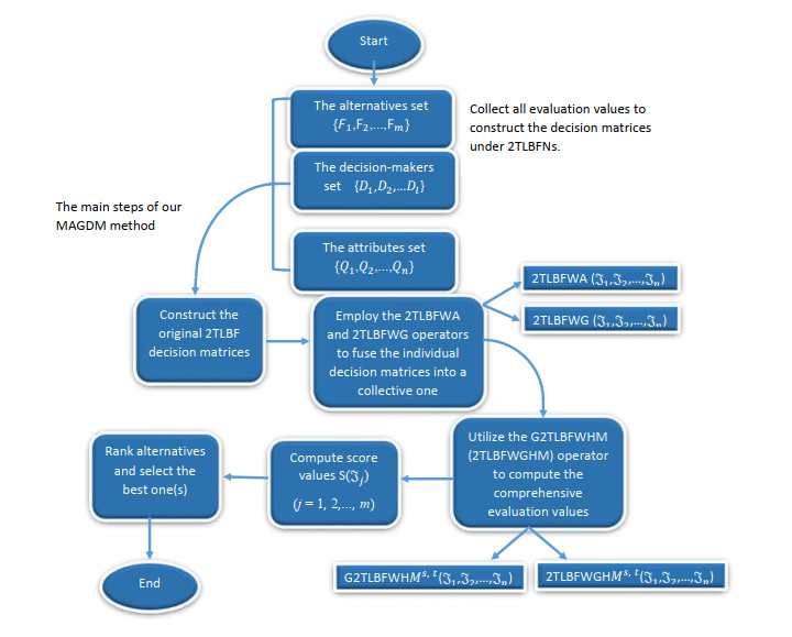
In this article, we introduce the 2-tuple linguistic bipolar fuzzy set (2TLBFS), a new strategy for dealing with uncertainty that incorporates a 2-tuple linguistic term into bipolar fuzzy set. The 2TLBFS is a better way to deal with uncertain and imprecise information in the decision-making environment. We elaborate the operational rules, based on which, the 2-tuple linguistic bipolar fuzzy weighted averaging (2TLBFWA) operator and the 2-tuple linguistic bipolar fuzzy weighted geometric (2TLBFWG) operator are presented to fuse the 2TLBF numbers (2TLBFNs). The Heronian mean (HM) operator, which can reflect the internal correlation between attributes and their influence on decision results, is integrated into the 2TLBF environment to analyze the effect of the correlation between decision factors on decision results. Initially, the generalized 2-tuple linguistic bipolar fuzzy Heronian mean (G2TLBFHM) operator and generalized 2-tuple linguistic bipolar fuzzy weighted Heronian mean (G2TLBFWHM) operator are proposed and properties are explained. Further, 2-tuple linguistic bipolar fuzzy geometric Heronian mean (2TLBFGHM) operator and 2-tuple linguistic bipolar weighted geometric Heronian mean (2TLBFWGHM) operator are proposed along with some of their desirable properties. Then, an approach to multi-attribute group decision-making (MAGDM) based on the proposed aggregation operators under the 2TLBF framework is developed. At last, a numerical illustration is provided for the selection of the best photovoltaic cell to demonstrate the use of the generated technique and exhibit its adequacy.
- 2-tuple linguistic bipolar fuzzy set,
- generalized HM operator,
- geometric HM operator,
- MAGDM,
- photovoltaic cells
Citation: Sumera Naz, Muhammad Akram, Mohammed M. Ali Al-Shamiri, Mohammed M. Khalaf, Gohar Yousaf. A new MAGDM method with 2-tuple linguistic bipolar fuzzy Heronian mean operators[J]. Mathematical Biosciences and Engineering, 2022, 19(4): 3843-3878. doi: 10.3934/mbe.2022177

Related Papers:

Abstract

In this article, we introduce the 2-tuple linguistic bipolar fuzzy set (2TLBFS), a new strategy for dealing with uncertainty that incorporates a 2-tuple linguistic term into bipolar fuzzy set. The 2TLBFS is a better way to deal with uncertain and imprecise information in the decision-making environment. We elaborate the operational rules, based on which, the 2-tuple linguistic bipolar fuzzy weighted averaging (2TLBFWA) operator and the 2-tuple linguistic bipolar fuzzy weighted geometric (2TLBFWG) operator are presented to fuse the 2TLBF numbers (2TLBFNs). The Heronian mean (HM) operator, which can reflect the internal correlation between attributes and their influence on decision results, is integrated into the 2TLBF environment to analyze the effect of the correlation between decision factors on decision results. Initially, the generalized 2-tuple linguistic bipolar fuzzy Heronian mean (G2TLBFHM) operator and generalized 2-tuple linguistic bipolar fuzzy weighted Heronian mean (G2TLBFWHM) operator are proposed and properties are explained. Further, 2-tuple linguistic bipolar fuzzy geometric Heronian mean (2TLBFGHM) operator and 2-tuple linguistic bipolar weighted geometric Heronian mean (2TLBFWGHM) operator are proposed along with some of their desirable properties. Then, an approach to multi-attribute group decision-making (MAGDM) based on the proposed aggregation operators under the 2TLBF framework is developed. At last, a numerical illustration is provided for the selection of the best photovoltaic cell to demonstrate the use of the generated technique and exhibit its adequacy.

References

[1]	Z. Ali, T. Mahmood, K. Ullah, Q. Khan, Einstein geometric aggregation operators using a novel complex interval-valued pythagorean fuzzy setting with application in green supplier chain management, Rep. Mech. Eng., 2 (2021), 105–134. https://doi.org/10.31181/rme2001020105t doi: 10.31181/rme2001020105t
[2]	R. Sahu, S. R. Dash, S. Das, Career selection of students using hybridized distance measure based on picture fuzzy set and rough set theory, Decis. Making Appl. Manage. Eng., 4 (2021), 104–126. https://doi.org/10.31181/dmame2104104s doi: 10.31181/dmame2104104s
[3]	L. A. Zadeh, Fuzzy sets, Inf. Control, 8 (1996), 338–353. https://doi.org/10.1016/S0019-9958(65)90241-X
[4]	K. T. Atanassov, Intuitionistic fuzzy sets, in Intuitionistic Fuzzy Sets, Physica, Heidelberg, (1999), 1–137. https://doi.org/10.1007/978-3-7908-1870-3_1
[5]	W. R. Zhang, Bipolar fuzzy sets and relations: a computational framework for cognitive modeling and multiagent decision analysis, in NAFIPS/IFIS/NASA'94. Proceedings of the First International Joint Conference of The North American Fuzzy Information Processing Society Biannual Conference. The Industrial Fuzzy Control and Intellige, (1994), 305–309. https://doi.org/10.1109/IJCF.1994.375115
[6]	M. Akram, U. Amjad, B. Davvaz, Decision-making analysis based on bipolar fuzzy N-soft information, Comput. Appl. Math., 40 (2021), 1–39. https://doi.org/10.1007/s40314-021-01570-y doi: 10.1007/s40314-021-01570-y
[7]	M. Zhao, G. Wei, C. Wei, Y. Guo, CPT-TODIM method for bipolar fuzzy multi-attribute group decision making and its application to network security service provider selection, Int. J. Intell. Syst., 36 (2021), 1943–1969. https://doi.org/10.1002/int.22367 doi: 10.1002/int.22367
[8]	M. Akram, M. Sarwar, W. A. Dudek, Graphs for the analysis of bipolar fuzzy information, Springer, 2021. https://doi.org/10.1007/978-981-15-8756-6
[9]	S. Poulik, G. Ghorai, Determination of journeys order based on graph's Wiener absolute index with bipolar fuzzy information, Inf. Sci., 545 (2021), 608–619. https://doi.org/10.1016/j.ins.2020.09.050 doi: 10.1016/j.ins.2020.09.050
[10]	M. Akram, T. Allahviranloo, W. Pedrycz, M. Ali, Methods for solving LR-bipolar fuzzy linear systems, Soft Comput., 25 (2021), 85–108. https://doi.org/10.1007/s00500-020-05460-z doi: 10.1007/s00500-020-05460-z
[11]	G. Ali, M. Akram, J. C. R. Alcantud, Attributes reductions of bipolar fuzzy relation decision systems, Neural Comput. Appl., 32 (2020), 10051–10071. https://doi.org/10.1007/s00521-019-04536-8 doi: 10.1007/s00521-019-04536-8
[12]	M. Akram, Shumaiza, A. N. Al-Kenani, Multi-criteria group decision-making for selection of green suppliers under bipolar fuzzy PROMETHEE process, Symmetry, 12 (2020), 77. https://doi.org/10.3390/sym12010077 doi: 10.3390/sym12010077
[13]	M. Akram, M. Arshad, Bipolar fuzzy TOPSIS and bipolar fuzzy ELECTRE-I methods to diagnosis, Comput. Appl. Math., 39 (2020), 1–21. https://doi.org/10.1007/s40314-019-0980-8 doi: 10.1007/s40314-019-0980-8
[14]	S. Naz, M. Akram, Novel decision-making approach based on hesitant fuzzy sets and graph theory, Comput. Appl. Math., 38 (2019), 1–26. https://doi.org/10.1007/s40314-019-0773-0 doi: 10.1007/s40314-019-0773-0
[15]	M. Akram, S. Naz, S. A. Edalatpanah, R. Mehreen, Group decision-making framework under linguistic q-rung orthopair fuzzy Einstein models, Soft Comput., 25 (2021), 10309–10334. https://doi.org/10.1007/s00500-021-05771-9 doi: 10.1007/s00500-021-05771-9
[16]	P. Liu, S. Naz, M. Akram, M. Muzammal, Group decision-making analysis based on linguistic q-rung orthopair fuzzy generalized point weighted aggregation operators, Int. J. Mach. Learn. Cybern., 2021 (2021), 1–24. https://doi.org/10.1007/s13042-021-01425-2 doi: 10.1007/s13042-021-01425-2
[17]	M. Akram, S. Naz, F. Ziaa, Novel decision-making framework based on complex q-rung orthopair fuzzy information, Scientia Iran., 2021 (2021), 1–34. https://doi.org/10.24200/SCI doi: 10.24200/SCI
[18]	S. Naz, M. Akram, S. Alsulami, F. Ziaa, Decision-making analysis under interval-valued q-rung orthopair dual hesitant fuzzy environment, Int. J. Comput. Intell. Syst., 14 (2021), 332–357. https://doi.org/10.2991/ijcis.d.201204.001 doi: 10.2991/ijcis.d.201204.001
[19]	M. Akram, S. Naz, F. Smarandache, Generalization of maximizing deviation and TOPSIS method for MADM in simplified neutrosophic hesitant fuzzy environment, Symmetry, 11 (8), 1058. https://doi.org/10.3390/sym11081058
[20]	H. Garg, S. Naz, F. Ziaa, Z. Shoukat, A ranking method based on Muirhead mean operator for group decision making with complex interval-valued q-rung orthopair fuzzy numbers, Soft Comput., 25 (2021), 14001–14027. https://doi.org/10.1007/s00500-021-06231-0
[21]	F. Herrera, L. Martínez, A 2-tuple fuzzy linguistic representation model for computing with words, IEEE Trans. Fuzzy Syst., 8 (2000), 746–752. https://doi.org/10.1109/91.890332 doi: 10.1109/91.890332
[22]	L. Martı, F. Herrera, An overview on the 2-tuple linguistic model for computing with words in decision making: extensions, applications and challenges, Inf. Sci., 207 (2012), 1–18. https://doi.org/10.1016/j.ins.2012.04.025 doi: 10.1016/j.ins.2012.04.025
[23]	Y. Zhang, G. Wei, Y. Guo, C. Wei, TODIM method based on cumulative prospect theory for multiple attribute group decision-making under 2-tuple linguistic pythagorean fuzzy environment, Int. J. Intell. Syst., 36 (2021), 2548–2571. https://doi.org/10.1002/int.22393 doi: 10.1002/int.22393
[24]	S. Faizi, W. Sacabun, S. Nawaz, A. Rehman, J. Watróbski, Best-worst method and Hamacher aggregation operations for intuitionistic 2-tuple linguistic sets, Expert Syst. Appl., 181 (2021), 115088. https://doi.org/10.1016/j.eswa.2021.115088 doi: 10.1016/j.eswa.2021.115088
[25]	A. Labella, B. Dutta, L. Martinez, An optimal best-worst prioritization method under a 2-tuple linguistic environment in decision making, Comput. Ind. Eng., 155 (2021), 107141. https://doi.org/10.1016/j.cie.2021.107141 doi: 10.1016/j.cie.2021.107141
[26]	M. Zhao, G. Wei, J. Wu, Y. Guo, TODIM method for multiple attribute group decision making based on cumulative prospect theory with 2-tuple linguistic neutrosophic sets, Int. J. Intell. Syst., 36 (2020), 1199–1222. https://doi.org/10.1002/int.22338 doi: 10.1002/int.22338
[27]	T. He, G. Wei, J. Wu, C. Wei, QUALIFLEX method for evaluating human factors in construction project management with Pythagorean 2-tuple linguistic information, J. Intell. Fuzzy Syst., 40 (2021), 1–12. https://doi.org/10.3233/JIFS-200379 doi: 10.3233/JIFS-200379
[28]	G. Beliakov, A. Pradera, T. Calvo, Aggregation Functions: Aguide for Practitioners, Springer, 2007.
[29]	S. Ayub, S. Abdullah, F. Ghani, M. Qiyas, M. Yaqub Khan, Cubic fuzzy Heronian mean dombi aggregation operators and their application on multi-attribute decision-making problems, Soft Comput., 25 (2021), 4175–4189. https://doi.org/10.1007/s00500-020-05512-4 doi: 10.1007/s00500-020-05512-4
[30]	M. Lin, X. Li, R. Chen, H. Fujita, J. Lin, Picture fuzzy interactional partitioned heronian mean aggregation operators: an application to MADM process, Artif. Intell. Rev., 2021 (2021), 1–38. https://doi.org/10.1007/s10462-021-09953-7 doi: 10.1007/s10462-021-09953-7
[31]	M. Deveci, D. Pamucar, I. Gokasar, Fuzzy power heronian function-based CoCoSo method for the advantage prioritization of autonomous vehicles in real-time traffic management, Sustainable Cities Soc., 69 (2021), 102846. https://doi.org/10.1016/j.scs.2021.102846 doi: 10.1016/j.scs.2021.102846
[32]	D. Pamucar, M. Behzad, D. Bozanic, M. Behzad, Decision making to support sustainable energy policies corresponding to agriculture sector: a case study in iran's caspian sea coastline, J. Cleaner Prod., 292 (2021), 125302. https://doi.org/10.1016/j.jclepro.2020.125302 doi: 10.1016/j.jclepro.2020.125302
[33]	H. Garg, Z. Ali, J. Gwak, T. Mahmood, S. Aljahdali, Some complex intuitionistic uncertain linguistic heronian mean operators and their application in multiattribute group decision making, J. Math., 2021 (2021). https://doi.org/10.1155/2021/9986704
[34]	P. Liu, Q. Khan, T. Mahmood, Group decision-making based on power Heronian aggregation operators under neutrosophic cubic environment, Soft Comput., 24 (2020), 1971–1997. https://doi.org/10.1007/s00500-019-04025-z doi: 10.1007/s00500-019-04025-z
[35]	F. Herrera, E. Herrera-Viedma, Linguistic decision analysis: steps for solving decision problems under linguistic information, Fuzzy Sets Syst., 115 (2000), 67–82. https://doi.org/10.1016/S0165-0114(99)00024-X doi: 10.1016/S0165-0114(99)00024-X
[36]	D. Yu, Intuitionistic fuzzy geometric Heronian mean aggregation operators, Appl. Soft Comput., 13 (2013), 1235–1246. https://doi.org/10.1016/j.asoc.2012.09.021 doi: 10.1016/j.asoc.2012.09.021
[37]	T. Hara, M. Uchiyama, S. E. Takahasi, A refinement of various mean inequalities, J. Inequalities Appl., 4 (1998), 387–395.
[38]	S. Wu, J. Wang, G. Wei, Y. Wei, Research on construction engineering project risk assessment with some 2-tuple linguistic neutrosophic Hamy mean operators, Sustainability, 10 (2018), 1536. https://doi.org/10.3390/su10051536 doi: 10.3390/su10051536
[39]	C. Maclaurin, A second letter to Martin Folkes, Esq.; concerning the roots of equations, with demonstration of other rules of algebra, Philos. Trans. R. Soc. Lond. Ser. A, 36 (1729), 59–96.
[40]	J. Qin, X. Liu, Approaches to uncertain linguistic multiple attribute decision making based on dual Maclaurin symmetric mean, J. Intell. Fuzzy Syst., 29 (2015), 171–186. https://doi.org/10.3233/IFS-151584 doi: 10.3233/IFS-151584

Reader Comments

Your name:*

Email:*
© 2022 the Author(s), licensee AIMS Press. This is an open access article distributed under the terms of the Creative Commons Attribution License (http://creativecommons.org/licenses/by/4.0)