Synchronization of the neurons coupled with sequential developing electrical and chemical synapses

Zhen Wang; Ramesh Ramamoorthy; Xiaojian Xi; Hamidreza Namazi; Zhen Wang; Ramesh Ramamoorthy; Xiaojian Xi; Hamidreza Namazi

doi:10.3934/mbe.2022088

Mathematical Biosciences and Engineering

2022, Volume 19, Issue 2: 1877-1890. doi: 10.3934/mbe.2022088

Previous Article Next Article

Research article Special Issues

Synchronization of the neurons coupled with sequential developing electrical and chemical synapses

1.
Xi'an Key Laboratory of Advanced Photo-electronics Materials and Energy Conversion Device, School of Science, Xijing University, Xi'an 710123, China
2.
Shaanxi International Joint Research Center for Applied Technology of Controllable Neutron Source School of Science, Xijing University, Xi'an 710123, China
3.
Centre for Artificial Intelligence, Chennai Institute of technology, Chennai, India
4.
School of Engineering, Monash University, Selangor, Malaysia
5.
College of Engineering and Science, Victoria University, Melbourne, Australia

Received: 30 October 2021 Accepted: 09 December 2021 Published: 20 December 2021

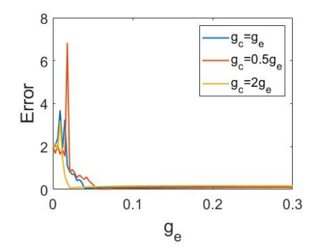
There is some evidence representing the sequential formation and elimination of electrical and chemical synapses in particular brain regions. Relying on this feature, this paper presents a purely mathematical modeling study on the synchronization among neurons connected by transient electrical synapses transformed to chemical synapses over time. This deletion and development of synapses are considered consecutive. The results represent that the transient synapses lead to burst synchronization of the neurons while the neurons are resting when both synapses exist constantly. The period of the transitions and also the time of presence of electrical synapses to chemical ones are effective on the synchronization. The larger synchronization error is obtained by increasing the transition period and the time of chemical synapses' existence.
- synchronization,
- neuronal network,
- transient electrical synapses,
- sequential synapses
Citation: Zhen Wang, Ramesh Ramamoorthy, Xiaojian Xi, Hamidreza Namazi. Synchronization of the neurons coupled with sequential developing electrical and chemical synapses[J]. Mathematical Biosciences and Engineering, 2022, 19(2): 1877-1890. doi: 10.3934/mbe.2022088

Related Papers:

Abstract

There is some evidence representing the sequential formation and elimination of electrical and chemical synapses in particular brain regions. Relying on this feature, this paper presents a purely mathematical modeling study on the synchronization among neurons connected by transient electrical synapses transformed to chemical synapses over time. This deletion and development of synapses are considered consecutive. The results represent that the transient synapses lead to burst synchronization of the neurons while the neurons are resting when both synapses exist constantly. The period of the transitions and also the time of presence of electrical synapses to chemical ones are effective on the synchronization. The larger synchronization error is obtained by increasing the transition period and the time of chemical synapses' existence.

References

[1]	S. Boccaletti, J. Kurths, G. Osipov, D. Valladares, C. Zhou, The synchronization of chaotic systems, Phys. Rep., 366 (2002), 1–101, doi: 10.1016/S0370-1573(02)00137-0. doi: 10.1016/S0370-1573(02)00137-0
[2]	A. L. Barabási, Network science, Philos. Trans. R. Soc. London Ser. A, 371 (2013), 20120375, doi: 10.1098/rsta.2012.0375. doi: 10.1098/rsta.2012.0375
[3]	S. Boccaletti, V. Latora, Y. Moreno, M. Chavez, D.-U. Hwang, Complex networks: Structure and dynamics, Phys. Rep., 424 (2006), 175–308, doi: 10.1016/j.physrep.2005.10.009. doi: 10.1016/j.physrep.2005.10.009
[4]	L. M. Pecora, T. L. Carroll, Synchronization in chaotic systems, Phys. Rev. Lett., 64 (1990), 821, doi: 10.1103/PhysRevLett.64.821. doi: 10.1103/PhysRevLett.64.821
[5]	A. Akgül, K. Rajagopal, A. Durdu, M. A. Pala, Ö. F. Boyraz, M. Z. Yildiz, A simple fractional-order chaotic system based on memristor and memcapacitor and its synchronization application, Chaos Solitons Fractals, 152 (2021), 111306, doi: 10.1016/j.chaos.2021.111306. doi: 10.1016/j.chaos.2021.111306
[6]	F. Drauschke, J. Sawicki, R. Berner, I. Omelchenko, E. Schöll, Effect of topology upon relay synchronization in triplex neuronal networks, Chaos, 30 (2020), 051104, doi: 10.1063/5.0008341. doi: 10.1063/5.0008341
[7]	L. M. Pecora, T. L. Carroll, Master stability functions for synchronized coupled systems, Phys. Rev. Lett., 80 (1998), 2109, doi: 10.1103/PhysRevLett.80.2109. doi: 10.1103/PhysRevLett.80.2109
[8]	F. Parastesh, C.-Y. Chen, H. Azarnoush, S. Jafari, B. Hatef, Synchronization patterns in a blinking multilayer neuronal network, Eur. Phys. J. Spec. Top., 228 (2019), 2465–2474, doi: 10.1140/epjst/e2019-800203-3. doi: 10.1140/epjst/e2019-800203-3
[9]	S. Rakshit, S. Majhi, B. K. Bera, S. Sinha, D. Ghosh, Time-varying multiplex network: Intralayer and interlayer synchronization, Phys. Rev. E, 96 (2017), 062308, doi: 10.1103/PhysRevE.96.062308. doi: 10.1103/PhysRevE.96.062308
[10]	I. V. Belykh, V. N. Belykh, M. Hasler, Blinking model and synchronization in small-world networks with a time-varying coupling, Phys. D, 195 (2004), 188–206, doi: 10.1016/j.physd.2004.03.013. doi: 10.1016/j.physd.2004.03.013
[11]	A. Buscarino, M. Frasca, M. Branciforte, L. Fortuna, J. C. Sprott, Synchronization of two Rössler systems with switching coupling, Nonlinear Dyn., 88 (2017), 673–683, doi: 10.1007/s11071-016-3269-0. doi: 10.1007/s11071-016-3269-0
[12]	J. J. Torres, I. Elices, J. Marro, Efficient transmission of subthreshold signals in complex networks of spiking neurons, PLoS One, 10 (2015), e0121156, doi: 10.1371/journal.pone.0121156. doi: 10.1371/journal.pone.0121156
[13]	A. Calim, T. Palabas, M. Uzuntarla, Stochastic and vibrational resonance in complex networks of neurons, Philos. Trans. R. Soc. London Ser. A, 379 (2021), 20200236, doi: 10.1098/rsta.2020.0236. doi: 10.1098/rsta.2020.0236
[14]	J. Ma, J. Tang, A review for dynamics of collective behaviors of network of neurons, Sci. China Technol. Sci., 58 (2015), 2038–2045, doi: 10.1007/s11431-015-5961-6. doi: 10.1007/s11431-015-5961-6
[15]	L. M. Ward, Synchronous neural oscillations and cognitive processes, Trends Cognit. Sci., 7 (2003), 553–559, doi: 10.1016/j.tics.2003.10.012. doi: 10.1016/j.tics.2003.10.012
[16]	K. Rajagopal, S. Jafari, A. Karthikeyan, A. Srinivasan, Effect of magnetic induction on the synchronizability of coupled neuron network, Chaos, 31 (2021), 083115, doi: 10.1063/5.0061406. doi: 10.1063/5.0061406
[17]	M. Shafiei, S. Jafari, F. Parastesh, M. Ozer, T. Kapitaniak, M. Perc, Time delayed chemical synapses and synchronization in multilayer neuronal networks with ephaptic inter-layer coupling, Commun. Nonlinear Sci. Numer. Simul., 84 (2020), 105175, doi: 10.1016/j.cnsns.2020.105175. doi: 10.1016/j.cnsns.2020.105175
[18]	P. Zhou, Z. Yao, J. Ma, Z. Zhu, A piezoelectric sensing neuron and resonance synchronization between auditory neurons under stimulus, Chaos Solitons Fractals, 145 (2021), 110751, doi: 10.1016/j.chaos.2021.110751. doi: 10.1016/j.chaos.2021.110751
[19]	I. Belykh, E. de Lange, M. Hasler, Synchronization of bursting neurons: What matters in the network topology, Phys. Rev. Lett., 94 (2005), 188101, doi: 10.1103/PhysRevLett.94.188101. doi: 10.1103/PhysRevLett.94.188101
[20]	S. Ostojic, N. Brunel, V. Hakim, Synchronization properties of networks of electrically coupled neurons in the presence of noise and heterogeneities, J. Comput. Neurosci., 26 (2009), 369–392, doi: 10.1007/s10827-008-0117-3. doi: 10.1007/s10827-008-0117-3
[21]	X. Sun, M. Perc, J. Kurths, Effects of partial time delays on phase synchronization in Watts-Strogatz small-world neuronal networks, Chaos, 27 (2017), 053113, doi: 10.1063/1.4983838. doi: 10.1063/1.4983838
[22]	C. Batista, S. Lopes, R. L. Viana, A. M. Batista, Delayed feedback control of bursting synchronization in a scale-free neuronal network, Neural Networks, 23 (2010), 114–124, doi: 10.1016/j.neunet.2009.08.005. doi: 10.1016/j.neunet.2009.08.005
[23]	L. Zhang, Y. Zhu, W. X. Zheng, Synchronization and state estimation of a class of hierarchical hybrid neural networks with time-varying delays, IEEE Trans. Neural Networks Learn. Syst., 27 (2015), 459–470, doi: 10.1109/TNNLS.2015.2412676. doi: 10.1109/TNNLS.2015.2412676
[24]	W. Qing-Yun, L. Qi-Shao, Time delay-enhanced synchronization and regularization in two coupled chaotic neurons, Chin. Phys. Lett., 22 (2005), 543, doi: 10.1088/0256-307X/22/3/007. doi: 10.1088/0256-307X/22/3/007
[25]	V. P. Zhigulin, M. I. Rabinovich, R. Huerta, H. D. Abarbanel, Robustness and enhancement of neural synchronization by activity-dependent coupling, Phys. Rev. E, 67 (2003), 021901, doi: 10.1103/PhysRevE.67.021901. doi: 10.1103/PhysRevE.67.021901
[26]	E. V. Pankratova, A. I. Kalyakulina, S. V. Stasenko, S. Y. Gordleeva, I. A. Lazarevich, V. B. Kazantsev, Neuronal synchronization enhanced by neuron–astrocyte interaction, Nonlinear Dyn., 97 (2019), 647–662, doi: 10.1007/s11071-019-05004-7. doi: 10.1007/s11071-019-05004-7
[27]	H. Fan, Y. Wang, H. Wang, Y.-C. Lai, X. Wang, Autapses promote synchronization in neuronal networks, Sci. Rep., 8 (2018), 1–13, doi: 10.1038/s41598-017-19028-9. doi: 10.1038/s41598-017-19028-9
[28]	A. E. Pereda, Electrical synapses and their functional interactions with chemical synapses, Nat. Rev. Neurosci., 15 (2014), 250–263, doi: 10.1038/nrn3708. doi: 10.1038/nrn3708
[29]	M. Golan, J. Boulanger-Weill, A. Pinot, P. Fontanaud, A. Faucherre, D. Gajbhiye, et al., Synaptic communication mediates the assembly of a self-organizing circuit that controls reproduction, Sci. Adv., 7 (2021), eabc8475, doi: 10.1126/sciadv.abc8475. doi: 10.1126/sciadv.abc8475
[30]	M. V. Bennett, Gap junctions as electrical synapses, J. Neurocytol., 26 (1997), 349–366, doi: 10.1023/A:1018560803261. doi: 10.1023/A:1018560803261
[31]	N. T. Carnevale, D. Johnston, Electrophysiological characterization of remote chemical synapses, J. Neurophysiol., 47 (1982), 606–621, doi: 10.1152/jn.1982.47.4.606. doi: 10.1152/jn.1982.47.4.606
[32]	A. O. Martin, G. Alonso, N. C. Guérineau, Agrin mediates a rapid switch from electrical coupling to chemical neurotransmission during synaptogenesis, J. Cell Biol., 169 (2005), 503–514, doi: 10.1083/jcb.200411054. doi: 10.1083/jcb.200411054
[33]	T. A. Zolnik, B. W. Connors, Electrical synapses and the development of inhibitory circuits in the thalamus, J. Physiol., 594 (2016), 2579–2592, doi: 10.1113/JP271880. doi: 10.1113/JP271880
[34]	S. Jabeen, V. Thirumalai, The interplay between electrical and chemical synaptogenesis, J. Neurophysiol., 120 (2018), 1914–1922, doi: 10.1152/jn.00398.2018. doi: 10.1152/jn.00398.2018
[35]	K. Kandler, E. Thiels, Flipping the switch from electrical to chemical communication, Nat. Neurosci., 8 (2005), 1633–1634, doi: 10.1038/nn1205-1633. doi: 10.1038/nn1205-1633
[36]	A. Marin-Burgin, F. J. Eisenhart, S. M. Baca, W. B. Kristan, K. A. French, Sequential development of electrical and chemical synaptic connections generates a specific behavioral circuit in the leech, J. Neurosci., 25 (2005), 2478–2489, doi: 10.1523/JNEUROSCI.4787-04.2005. doi: 10.1523/JNEUROSCI.4787-04.2005
[37]	T. M. Szabo, D. S. Faber, M. J. Zoran, Transient electrical coupling delays the onset of chemical neurotransmission at developing synapses, J. Neurosci., 24 (2004), 112–120, doi: 10.1523/JNEUROSCI.4336-03.2004. doi: 10.1523/JNEUROSCI.4336-03.2004
[38]	K. L. Todd, W. B. Kristan, K. A. French, Gap junction expression is required for normal chemical synapse formation, J. Neurosci., 30 (2010), 15277–15285, doi: 10.1523/JNEUROSCI.2331-10.2010. doi: 10.1523/JNEUROSCI.2331-10.2010
[39]	Y. Wang, J. E. Rubin, Complex bursting dynamics in an embryonic respiratory neuron model, Chaos, 30 (2020), 043127, doi: 10.1063/1.5138993. doi: 10.1063/1.5138993

Reader Comments

Your name:*

Email:*
© 2022 the Author(s), licensee AIMS Press. This is an open access article distributed under the terms of the Creative Commons Attribution License (http://creativecommons.org/licenses/by/4.0)