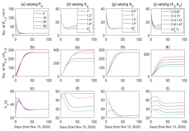
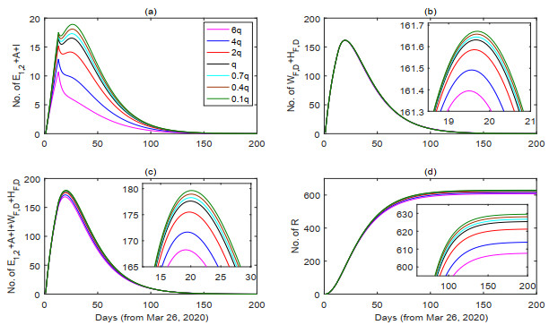
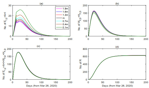
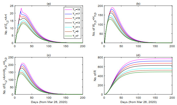
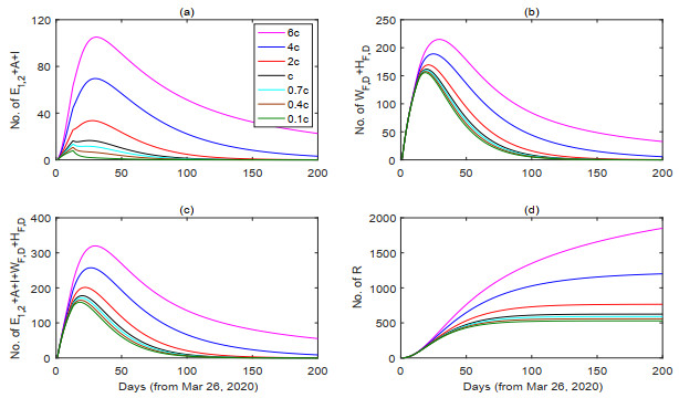
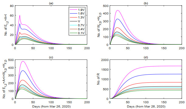
Since the outbreak of COVID-19 in Wuhan, China in December 2019, it has spread quickly and become a global pandemic. While the epidemic has been contained well in China due to unprecedented public health interventions, it is still raging or not yet been restrained in some neighboring countries. Chinese government adopted a strict policy of immigration diversion in major entry ports, and it makes Suifenhe port in Heilongjiang Province undertook more importing population. It is essential to understand how imported cases and other key factors of screening affect the epidemic rebound and its mitigation in Heilongjiang Province. Thus we proposed a time switching dynamical system to explore and mimic the disease transmission in three time stages considering importation and control. Cross validation of parameter estimations was carried out to improve the credibility of estimations by fitting the model with eight time series of cumulative numbers simultaneous. Simulation of the dynamics shows that illegal imported cases and imperfect protection in hospitals are the main reasons for the second epidemic wave, the actual border control intensities in the province are relatively effective in early stage. However, a long-term border closure may cause a paradox phenomenon such that it is much harder to restrain the epidemic. Hence it is essential to design an effective border reopening strategy for long-term border control by balancing the limited resources on hotel rooms for quarantine and hospital beds. Our results can be helpful for public health to design border control strategies to suppress COVID-19 transmission.
Citation: Xianghong Zhang, Yunna Song, Sanyi Tang, Haifeng Xue, Wanchun Chen, Lingling Qin, Shoushi Jia, Ying Shen, Shusen Zhao, Huaiping Zhu. Models to assess imported cases on the rebound of COVID-19 and design a long-term border control strategy in Heilongjiang Province, China[J]. Mathematical Biosciences and Engineering, 2022, 19(1): 1-33. doi: 10.3934/mbe.2022001
Since the outbreak of COVID-19 in Wuhan, China in December 2019, it has spread quickly and become a global pandemic. While the epidemic has been contained well in China due to unprecedented public health interventions, it is still raging or not yet been restrained in some neighboring countries. Chinese government adopted a strict policy of immigration diversion in major entry ports, and it makes Suifenhe port in Heilongjiang Province undertook more importing population. It is essential to understand how imported cases and other key factors of screening affect the epidemic rebound and its mitigation in Heilongjiang Province. Thus we proposed a time switching dynamical system to explore and mimic the disease transmission in three time stages considering importation and control. Cross validation of parameter estimations was carried out to improve the credibility of estimations by fitting the model with eight time series of cumulative numbers simultaneous. Simulation of the dynamics shows that illegal imported cases and imperfect protection in hospitals are the main reasons for the second epidemic wave, the actual border control intensities in the province are relatively effective in early stage. However, a long-term border closure may cause a paradox phenomenon such that it is much harder to restrain the epidemic. Hence it is essential to design an effective border reopening strategy for long-term border control by balancing the limited resources on hotel rooms for quarantine and hospital beds. Our results can be helpful for public health to design border control strategies to suppress COVID-19 transmission.

| [1] | Sina News. Update on the outbreak of Covid-19 at 24: 00, 18 March, 2020. Available from: http://news.sina.com.cn/zx/2020-03-19/doc-iimxxsth0137436.shtml (accessed on 18 Mar 2020). |
| [2] | Heilongjiang Daily. CCTV news 1+1: focuses on Suifenhe, China, 2020. Available from: http://www.hlj.gov.cn/zwfb/system/2020/04/14/010923836.shtml (accessed on 14 Apr 2020). |
| [3] | CAAC. Notice on the continued reduction of international passenger flights during the epidemic prevention and control period, 2020. Available from: http://www.caac.gov.cn/XXGK/XXGK/TZTG/202003/t20200326_201746.html (accessed on 26 Mar 2020). |
| [4] | CAAC. Notice of civil Aviation Administration on adjustment of international passenger flights, Civil aviation administration of China, 2020. Available from: http://www.caac.gov.cn/XXGK/XXGK/TZTG/202006/t20200604_202928.html (accessed on 4 Jun 2020). |
| [5] | Sina News. The Civil Aviation Administration responded that international flights have been redirected to 12 entry points: Beijing Airport has more than 200 inbound flights from 33 countries every week, 2020. Available from: http://finance.sina.com.cn/roll/2020-03-23/doc-iimxxsth1242997.shtml (accessed on 23 Mar 2020). |
| [6] | Heilongjiang Municipal Government. The Suifenhe-Bologanichny Port Passenger Inspection Channel was temporarily closed, 2020. Available from: https://www.hlj.gov.cn/n200/2020/0408/c35-10923381.html (accessed on 8 Apr 2020). |
| [7] | Suifenhe Municipal People's Government. Notice No.19 of Suifenhe Epidemic Prevention and Control Headquarters, 2020. Available from: http://www.suifenhe.gov.cn/contents/1962/80492.html (accessed on 9 Apr 2020). |
| [8] | Suifenhe Municipal People's Government. Document No.9: Suifenhe City shall respond to the control measures of 'Nine Stricts and One Protection' for CoviD-19 epidemic prevention and export prevention and control, 2020. Available from: http://www.suifenhe.gov.cn/contents/1962/80547.html (accessed on 12 Apr 2020). |
| [9] | Suifenhe Municipal People's Government. Suifenhe epidemic prevention and control headquarters twenty-first notice, 2020. Available from: http://www.suifenhe.gov.cn/contents/1962/80548.html (accessed on 12 Apr 2020). |
| [10] | Heilongjiang Public Security Department. Heilongjiang issued Notice No.14: The first place of entry is the place of quarantine, 2020. Available from: https://mp.weixin.qq.com/s/FXArnr4pyo9qAXUgsH5leA (accessed on 2 Apr 2020). |
| [11] | Health Commission of Heilongjiang Province. Latest outbreak report, 2020. Available from: http://wsjkw.hlj.gov.cn/pages/5fd2a7e712c15bde3d36385a (accessed on 11 Dec 2020). |
| [12] | Health Commission of Heilongjiang Province. Latest outbreak report, 2021. Available from: http://wsjkw.hlj.gov.cn/pages/6008c1ff12c15b4f69f68e3c (accessed on 21 Jan 2020). |
| [13] | X. Yu, Modelling Return of the Epidemic: Impact of Population Structure, Asymptomatic Infection, Case Importation and Personal Contacts, Travel Med. Infect. Di., 37 (2020), 1-8. doi: 10.1016/j.tmaid.2020.101858. |
| [14] | M. Kraemer, C. Yang, B. Gutierrez, C. H. Wu, B. Klein, D. M. Pigott, et al., The effect of human mobility and control measures on the COVID-19 epidemic in China, Science, 368 (2020), 493-497. doi: 10.1126/science.abb4218. |
| [15] | H. Sun, B. Dickens, A. Cook, H. Clapham, Importations of COVID-19 into African countries and risk of onward spread, BMC Infect. Dis., 20 (2020), 1-13. doi: 10.1186/s12879-020-05323-w. |
| [16] | T. Sun, D. Weng, Estimating the effects of asymptomatic and imported patients on COVID-19 epidemic using mathematical modeling, J. Med. Virol., 92 (2020), 1995-2003. doi: 10.1002/jmv.25939. |
| [17] | Z. Hu, Q. Cui, J. Han, X. Wang, E. Wei, Z. Teng, Evaluation and prediction of the COVID-19 variations at different input population and quarantine strategies, a case study in Guangdong province, China, Int. J. Infect. Dis., 95 (2020), 231-240. doi: 10.1016/j.ijid.2020.04.010. |
| [18] | M. Hossain, A. Junus, X. Zhu, P. Jia, T. Wen, D. Pfeiffer, et al., The effects of border control and quarantine measures on the spread of COVID-19, Epidemics 32 (2020), 100397. doi: 10.1016/j.epidem.2020.100397. |
| [19] | T. Chen, J. Rui, Q. Wang, Z. Zhao, J. Cui, L. Yin, A mathematical model for simulating the phase-based transmissibility of a novel coronavirus, Infect. Dis. Poverty, 9 (2020), 1-8. doi: 10.1186/s40249-020-00640-3. |
| [20] | I. Coopera, A. Mondal, C. Antonopoulos, Dynamic tracking with model-based forecasting for the spread of the COVID-19 pandemic, Chaos Soliton. Fract., 139 (2020), 110298. doi: 10.1016/j.chaos.2020.110298. |
| [21] | Q. Li, Y. Xiao, J. Wu, Modelling COVID-19 epidemic with time delay and analyzing the strategy of confirmed cases-driven contact tracing followed by quarantine, Acta Math. Appl. Sin., 43 (2020), 238-250. (in Chinese) |
| [22] | L. Zou, S. Ruan, A patch model of COVID-19: the effects of containment on chongqing, Acta Math. Appl. Sin., 43 (2020), 310-323. (in Chinese) |
| [23] | H. Loeffler-Wirth, M. Schmidt, H. Binder, Covid-19 transmission trajectories$-$monitoring the pandemic in the worldwide context, Viruses, 12 (2020), 777. doi: 10.3390/v12070777. |
| [24] | J. Hellewell, S. Abbot, A. Gimma, N. Bosse, C. Jarvis, T. Russell, et al., Feasibility of controlling COVID-19 outbreaks by isolation of cases and contacts, Lancet Glob. Health, 8 (2020), e488-e496. doi: 10.1016/S2214-109X(20)30074-7. |
| [25] | G. Giordano, F. Blanchini, R. Bruno, P. Colaneri, A. Di Filippo, A. Di Matteo, et al., Modelling the COVID-19 epidemic and implementation of population-wide interventions in Italy, Nat. Med., 26 (2020), 855-885. doi: 10.1038/s41591-020-0883-7. |
| [26] | S. Saha, G. Samanta, J. Nieto, Epidemic model of COVID-19 outbreak by inducing behavioural response in population, Nonlinear Dynam., 102 (2020), 455-487. doi: 10.1007/s11071-020-05896-w. |
| [27] | F. Ndaïrou, I. Area, J. Nieto, D. Torres, Mathematical modeling of COVID-19 transmission dynamics with a case study of Wuhan, Chaos Soliton. Fract., 135 (2020), 109846. doi: 10.1016/j.chaos.2020.109846. |
| [28] | K. Bubar, K. Reinholt, S. Kissler, M. Lipsitch, S. Cobey, Y. Grad, et al., Model-informed COVID-19 vaccine prioritization strategies by age and serostatus, Science, 371 (2021), 916-921. doi: 10.1126/science.abe6959. |
| [29] | C. Kerr, R. Stuart, D. Mistry, R. Abeysuriya, K. Rosenfeld, G. Hart, et al., Covasim: an agent-based model of COVID-19 dynamics and interventions, PLOS Comput. Biol., 17 (2021), e1009149. doi: 10.1371/journal.pcbi.1009149. |
| [30] | I. Baba, A. Yusuf, K. Nisar, A. Abdel-Aty, T. Nofal, Mathematical model to assess the imposition of lockdown during COVID-19 pandemic, Results Phys., 20 (2021), 103716. doi: 10.1016/j.rinp.2020.103716. |
| [31] | S. Nadim, I. Ghosh, J. Chattopadhyay, Short-term predictions and prevention strategies for COVID-19: a model-based study, Appl. Math. and Comput., 404 (2021), 126251. doi: 10.1016/j.amc.2021.126251. |
| [32] | P. Driessche, J. Watmough, Reproduction numbers and sub-threshold endemic equilibria for compartmental models of disease transmission, Math. Biosci., 180 (2002), 29-48. doi: 10.1016/s0025-5564(02)00108-6. |
| [33] | Q. Li, B. Tang, N. Bragazzi, Y. Xiao, J. Wu, Modeling the impact of mass influenza vaccination and public health interventions on covid-19 epidemics with limited detection capability, Math. Biosci., 325 (2020), 108378. doi: 10.1016/j.mbs.2020.108378. |
| [34] | B. Tang, X. Wang, Q. Li, N. Bragazzi, S. Tang, Y. Xiao, et al., Estimation of the Transmission Risk of the 2019-nCoV and Its Implication for Public Health Interventions, J. Clin. Med., 9 (2020), 462. doi: 10.3390/jcm9020462. |
| [35] | S. Tang, Z. Xu, X. Wang, X. Feng, Y. Xiao, Y. Chen, et al., When will be the resumption of work in wuhan and its surrounding areas during covid-19 epidemic? A data-driven network modeling analysis, Scientia Sinica Mathematica, 50 (2020), 969-978. doi: 10.1360/SSM-2020-0037 |
| [36] | A. Morton, B. Finkenstadt, Discrete time modelling of disease incidence time series by using Markov chain Monte Carlo methods. Discrete time modelling of disease incidence time series by using markov chain monte carlo methods, J. R. Stat. Soc. C-Appl., 54 (2005), 575-594. doi: 10.1111/j.1467-9876.2005.05366.x. |
| [37] | M. Keeling, M. Tildesley, B. Atkins, B. Penman, E. Southall, GirlGuyver-Fletcher, et al., The impact of school reopening on the spread of COVID-19 in England, Philos. T. R. Soc. B., 376 (2021), 20200261. doi: 10.1098/rstb.2020.0261. |
Figures(14) / Tables(4)

Xianghong Zhang, Yunna Song, Sanyi Tang, Haifeng Xue, Wanchun Chen, Lingling Qin, Shoushi Jia, Ying Shen, Shusen Zhao, Huaiping Zhu. Models to assess imported cases on the rebound of COVID-19 and design a long-term border control strategy in Heilongjiang Province, China[J]. Mathematical Biosciences and Engineering, 2022, 19(1): 1-33. doi: 10.3934/mbe.2022001


 DownLoad: