ECG compression with Douglas-Peucker algorithm and fractal interpolation

Hichem Guedri; Abdullah Bajahzar; Hafedh Belmabrouk; Hichem Guedri; Abdullah Bajahzar; Hafedh Belmabrouk

doi:10.3934/mbe.2021176

Mathematical Biosciences and Engineering

2021, Volume 18, Issue 4: 3502-3520. doi: 10.3934/mbe.2021176

Previous Article Next Article

Research article

ECG compression with Douglas-Peucker algorithm and fractal interpolation

1.
Electronics and Microelectronics Laboratory, Physics Department, Faculty of Sciences, Monastir University, Monastir 5019, Tunisia
2.
Department of Computer Science and Information, College of Science, Majmaah University, Zulfi 11932, Saudi Arabia
3.
Department of Physics, College of Science Zulfi, Majmaah University, Zulfi 11932, Saudi Arabia

Academic Editor: Eugene Kashdan

Received: 17 January 2021 Accepted: 28 March 2021 Published: 21 April 2021

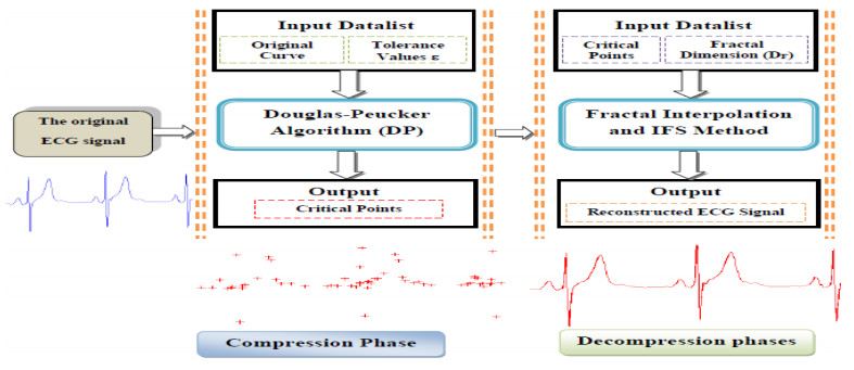
In this paper, we propose a new ECG compression method using the fractal technique. The proposed approaches utilize the fact that ECG signals are a fractal curve. This algorithm consists of three steps: First, the original ECG signals are processed and they are converted into a 2-D array. Second, the Douglas-Peucker algorithm (DP) is used to detect critical points (compression phase). Finally, we used the fractal interpolation and the Iterated Function System (IFS) to generate missing points (decompression phase). The proposed (suggested) methodology is tested for different records selected from PhysioNet Database. The obtained results showed that the proposed method has various compression ratios and converges to a high value. The average compression ratios are between 3.19 and 27.58, and also, with a relatively low percentage error (PRD), if we compare it to other methods. Results depict also that the ECG signal can adequately retain its detailed structure when the PSNR exceeds 40 dB.
- electrocardiogram (ECG),
- compression method,
- Douglas-Peucker algorithm (DP),
- fractal interpolation,
- Iterated Function System (IFS)
Citation: Hichem Guedri, Abdullah Bajahzar, Hafedh Belmabrouk. ECG compression with Douglas-Peucker algorithm and fractal interpolation[J]. Mathematical Biosciences and Engineering, 2021, 18(4): 3502-3520. doi: 10.3934/mbe.2021176

Related Papers:

Abstract

In this paper, we propose a new ECG compression method using the fractal technique. The proposed approaches utilize the fact that ECG signals are a fractal curve. This algorithm consists of three steps: First, the original ECG signals are processed and they are converted into a 2-D array. Second, the Douglas-Peucker algorithm (DP) is used to detect critical points (compression phase). Finally, we used the fractal interpolation and the Iterated Function System (IFS) to generate missing points (decompression phase). The proposed (suggested) methodology is tested for different records selected from PhysioNet Database. The obtained results showed that the proposed method has various compression ratios and converges to a high value. The average compression ratios are between 3.19 and 27.58, and also, with a relatively low percentage error (PRD), if we compare it to other methods. Results depict also that the ECG signal can adequately retain its detailed structure when the PSNR exceeds 40 dB.

References

[1]	C. C. Chen, C. W. Chen, C. W. Hsieh, Noise-resistant CECG using novel capacitive electrodes, Sensors, 20 (2020), 1-17. doi: 10.1109/JSEN.2020.3010656
[2]	J. C. Carrillo-Alarcón, L. A. Morales-Rosales, H. Rodríguez-Rángel, M. Lobato-Báez, A. Muñoz, I. Algredo-Badillo, A metaheuristic optimization approach for parameter estimation in arrhythmia classification from unbalanced data, Sensors, 20 (2020), 1-29. doi: 10.3390/s20174952
[3]	M. Yin, R. Tang, M. Liu, K. Han, X. Lv, Influence of optimization design based on artificial intelligence and internet of things on the electrocardiogram monitoring system, J. Healthc. Eng., 2020 (2020), 1-8.
[4]	N. Reljin, J. Lazaro, M. B. Hossain, Y. S. Noh, C. H. Cho, K. H Chon, Using the redundant convolutional encoder-decoder to denoise QRS complexes in ECG signals recorded with an armband wearable device, Sensors, 20 (2020), 1-15.
[5]	Q. Shen, H. Gao, Y. Li, Q. Sun, M. Chen, An Open-Access arrhythmia database of wearable electrocardiogram, J. Med. Biol. Eng., 40 (2020), 564-574. doi: 10.1007/s40846-020-00554-3
[6]	M. F. Pérez-Gutiérrez, J. J. Sánchez-Muñoz, M. Erazo-Rodas, A. Guerrero-Curieses, E. Everss, A. Quesada-Dorador, Spectral analysis and mutual information estimation of left and right intracardiac electrograms during ventricular fibrillation, Sensors, 20 (2020), 1-20. doi: 10.1109/JSEN.2020.3010656
[7]	R. Caulier-Cisterna, M. Sanromán-Junquera, S. Muñoz-Romero, M. Blanco-Velasco, Spatial-temporal signals and clinical indices in electrocardiographic imaging (I): preprocessing and bipolar potentials, Sensors, 20 (2020), 1-28. doi: 10.3390/s20072153
[8]	R. Ranjan, V. K. Giri, A unified approach of ECG signal analysis, Int. J. Soft. Comput. Eng., 2 (2012), 5-10.
[9]	L. Rebollo-Neira, Effective high compression of ECG signals at low level distortion, Sci. Rep., 9 (2019), 1-12.
[10]	K. Ranjeet, A. Kumar, R. K. Pandey, ECG signal compression using different techniques, In Unnikrishnan S., Surve S., Bhoir D. (eds) Advances in Computing, Communication and Control. ICAC3 2011. Communications in Computer and Information Science, Springer, Berlin, Heidelberg, 125 (2011).
[11]	M. Abo-Zahhad, A. F. Al-Ajlouni, S. M. Ahmed, R. J. Schilling, A new algorithm for the compression of ECG signals based on mother wavelet parameterization and best-threshold levels selection, Digit. Signal Process., 23 (2013), 1002-1011. doi: 10.1016/j.dsp.2012.11.005
[12]	M. Abo-Zahhad, S. M. Ahmed, A. Zakaria, An efficient technique for compressing ECG signals using QRS detection, estimation, and 2D DWT coefficients thresholding, Model. Simulat. Eng., 2012 (2012), 1-10.
[13]	M. Abo-Zahhad, B. A. Rajoub, An effective coding technique for the compression of one-dimensional signals using wavelet transforms, Med. Eng. Phys., 24 (2002), 185-199. doi: 10.1016/S1350-4533(02)00004-8
[14]	P. Cebrian, J. C. Moure, GPU-accelerated RDP algorithm for data segmentation, In Krzhizhanovskaya V. et al. (eds) Computational Science-ICCS 2020. ICCS 2020. Lecture Notes in Computer Science, Springer, Cham, 12137 (2020).
[15]	X. Wang, W. Yang, Y. Liu, R. Sun, J. Hu, Segmented Douglas-Peucker algorithm based on the node importance, KSⅡ Trans. Internet. Inf. Syst., 14 (2020), 1562-1578.
[16]	L. Zhao, G. Shi, A method for simplifying ship trajectory based on improved Douglas-Peucker algorithm, Ocean. Eng., 166 (2018), 37-46. doi: 10.1016/j.oceaneng.2018.08.005
[17]	Y. Q. Zhang, G. Y. Shi, S. Li, S. K. Zhang, Vessel trajectory online multi-dimensional simplification algorithm, J. Navig., 73 (2020), 342-363. doi: 10.1017/S037346331900064X
[18]	J. Liu, H. Li, Z. Yang, K. Wu, Y. Liu, R. W. Liu, Adaptive Douglas-Peucker algorithm with automatic thresholding for AIS-Based vessel trajectory compression, IEEE Access, 7 (2019), 150677-150692. doi: 10.1109/ACCESS.2019.2947111
[19]	S. Lakhera, T. Praveena, Visual analysis using modified Ramer-Douglas-Peucker algorithm on time series data, Int. Res. J. Eng. Technol., 07 (2020), 4225-4229.
[20]	R. B. McMaster, Automated line generalisation, Cartographica, 24 (1987), 74-111.
[21]	White, E. R., Assessment of line-generalization algorithms using characteristic point, Am. Cartographer, 12 (1985), 17-27.
[22]	J. S. Marino, Identification of characteristic points along naturally occurring lines. an empirical study, Can. cart/Toronto., 16 (1979), 70-80.
[23]	S. Dillon, V. Drakopoulos, On self‐affine and self‐similar graphs of fractal interpolation functions generated from iterated function systems, Fract. Anal. Appl. Health Sci. Soc. Sci., Fernando Brambila, 9 (2017), 187-204.
[24]	R. A. Al-Jawfi, Approximation of fractal interpolation using artificial neural network, J. Eng. Appl. Sci., 15 (2020), 1337-1340. doi: 10.36478/jeasci.2020.1337.1340
[25]	S. I. Ri, New types of fractal interpolation surfaces, Chaos Soliton. Fract., 119 (2019), 291-297. doi: 10.1016/j.chaos.2019.01.010
[26]	S. I. Ri, A new nonlinear bivariate fractal interpolation function, Fractals, 26 (2018), 1-24.
[27]	V. Drakopoulos, P. Manousopoulos, On non-tensor product bivariate fractal interpolation surfaces on rectangular grids, Mathematics, 8 (2020), 1-19.
[28]	P. R. Massopust, Fractal Functions, Fractal Surfaces and Wavelets, 2^nd edition, San Diego: Academic Press, 2016.
[29]	N. Vijender, A. K. B. Chand, Shape preserving affine fractal interpolation surfaces, Nonlinear Stud., 21(2014), 175-190.
[30]	M. A. Navascués, A. K. B. Chand, V. P. Veedu, M. V. Sebastián, Fractal interpolation functions: a short survey, Appl. Math., 5 (2014), 1834-1841. doi: 10.4236/am.2014.512176
[31]	M. F. Barnsley, P. R. Massopust, Bilinear fractal interpolation and box dimension, J. Approx. Theory, 192 (2015), 362-378. doi: 10.1016/j.jat.2014.10.014
[32]	C. Corda, M. FatehiNia, M. Molaei, Y. Sayyari, Entropy of iterated function systems and their relations with black holes and bohr-like black holes entropies, Entropy, 20 (2018), 1-17.
[33]	H. Y. Wang, J. S. Yu, J. S. Yu, Fractal interpolation functions with variable parameters and their analytical properties, J. Approx. Theory, 175 (2013), 1-18. doi: 10.1016/j.jat.2013.07.008
[34]	M. Rahman, A. H. M. Z. Karim, A. Al-Mahmud, S. N. Rahman, Detection of abnormality in electrocardiogram (ECG) signals based on Katz's and Higuchi's method under fractal dimensions, Comput. Biol. Bioinform., 4 (2016), 27-36. doi: 10.11648/j.cbb.20160404.11
[35]	H. Namazi, V. Kulish, Fractal based analysis of the influence of odorants on heart activity, Sci. Rep., 6 (2016), 1-8. doi: 10.1038/s41598-016-0001-8
[36]	L. Rebollo-Neira, Effective high compression of ECG signals at low level distortion, Sci. Rep., 9 (2019), 1-12
[37]	A. R. Garg, M. K. Mathur, Use of self organizing map to obtain ECG data templates for its compression and reconstruction, Int. J. Comput. Appl., 137 (2016), 26-33.
[38]	T. I. Mohammadpour, M. R. K. Mollaei, ECG compression with thresholding of 2-D wavelet transform coefficients and run length coding, Eur. J. Sci. Res., 27 (2009), 248-257.
[39]	M. Moazami-Goudarzi, A. Taheri, M. Pooyan, Efficient method for ECG compression using two dimensional multiwavelet transform, Int. J. Inf. Technol., 2 (2005), 257-263.
[40]	H. H. Chou, Y. J. Chen, Y. C. Shiau, T. S. Kuo, An effective and efficient compression algorithm for ECG signals with irregular periods, IEEE. Trans. Biomed. Eng., 53 (2006), 1198-1205. doi: 10.1109/TBME.2005.863961
[41]	R. Kumar, A. Kumar, G. K. Singh, H. N. Lee, Efficient compression technique based on temporal modelling of ECG signal using principle component analysis, IET Sci. Meas. Technol., 11 (2017), 346-353. doi: 10.1049/iet-smt.2016.0360
[42]	R. Kumar, A. Kumar, G. Akhil, A. Singh, S. N. H. Jafri, Computationally efficient method for ECG signal compression based on modified SPIHT technique, Int. J. Biomed. Eng. Technol., 15 (2014), 173-188. doi: 10.1504/IJBET.2014.062746
[43]	K. Ranjeet, A. Kumar, Rajesh K. Pandey, An efficient compression system for ECG signal using QRS periods and CAB technique based on 2D DWT and huffman coding, Control, Autom., Robot. Embedded Syst. (CARE), 2013.
[44]	R. Kumar, A. R. Verma, B. Gupta, S. Kumar, Dual-tree sparse decomposition of DWT filters for ECG signal compression and HRV analysis, Augment. Hum. Res., 6 (2021), 1-8. doi: 10.1007/s41133-020-00039-7
[45]	R. Gupta, Quality aware compression of electrocardiogram using principal component analysis, J. Med. Syst., 40 (2016), 1-11. doi: 10.1007/s10916-015-0365-5
[46]	J. Liu, F. Chen, D. Wang, Data compression based on stacked RBM-AE model for wireless sensor networks, Sensors, 18 (2018), 1-19. doi: 10.1109/JSEN.2018.2870228
[47]	T. Y. Liu, K. J. Lin, H. C. Wu, ECG data encryption then compression using singular value decomposition, IEEE J. Biomed. Health Informat., 22 (2018), 707-713. doi: 10.1109/JBHI.2017.2698498
[48]	S. K. Mukhopadhyay, M. O. Ahmad, M. N. S. Swamy, An ECG compression algorithm with guaranteed reconstruction quality based on optimum truncation of singular values and ASCⅡ character encoding, Biomed. Signal Process. Control., 44 (2018), 288-306. doi: 10.1016/j.bspc.2018.05.005
[49]	Z. Peng, G. Wang, H. Jiang, S. Meng, Research and imp rovement of ECG compression algorithm based on EZW, Comput. Meth. Prog. Bio., 145 (2017), 157-166. doi: 10.1016/j.cmpb.2017.04.015
[50]	F. Wang, Q. Ma, W. Liu, S. Chang, novel ECG signal compression method using spindle convolutional auto-encoder, Comput. Meth. Prog. Bio., 175 (2019), 139-150. doi: 10.1016/j.cmpb.2019.03.019
[51]	O. Yildirim, R. S. Tan, U. R. Acharya, An efficient compression of ECG signals using deep convolutional autoencoders, Cognit. Syst. Res., 52 (2018), 198-211. doi: 10.1016/j.cogsys.2018.07.004
[52]	Research Resource for Complex Physiologic Signals (PhysioNet), Available online: https://physionet.org/about/database/#restricted.
[53]	A. L. Goldberger, L. A. N. Amaral, L. Glass, J. M. Hausdorff, P. C. Ivanov, PhysioBank, PhysioToolkit, and PhysioNet: components of a new research resource for complex physiologic signals, Circulation, 101 (2000), e215-e220.
[54]	M. B. Hossain, S. K. Bashar, A. J. Walkey, D. D. McManus, K. H. Chon, An accurate QRS complex and P wave detection in ECG signals using complete ensemble empirical mode decomposition with adaptive noise approach, IEEE Access, 7 (2019), 128869-128880. doi: 10.1109/ACCESS.2019.2939943

Reader Comments

Your name:*

Email:*
© 2021 the Author(s), licensee AIMS Press. This is an open access article distributed under the terms of the Creative Commons Attribution License (http://creativecommons.org/licenses/by/4.0)