Mathematical modeling and dynamic analysis of SIQR model with delay for pandemic COVID-19

Hongfan Lu; Yuting Ding; Silin Gong; Shishi Wang; Hongfan Lu; Yuting Ding; Silin Gong; Shishi Wang

doi:10.3934/mbe.2021159

Mathematical Biosciences and Engineering

2021, Volume 18, Issue 4: 3197-3214. doi: 10.3934/mbe.2021159

Previous Article Next Article

Research article Special Issues

Mathematical modeling and dynamic analysis of SIQR model with delay for pandemic COVID-19

Department of Mathematics, Northeast Forestry University, Harbin, 150040, China

Academic Editor: Cristiana Silva

Received: 24 February 2021 Accepted: 02 April 2021 Published: 06 April 2021

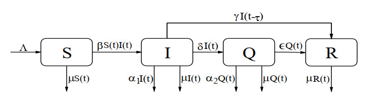
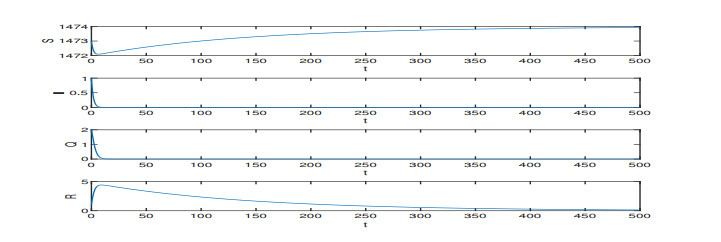
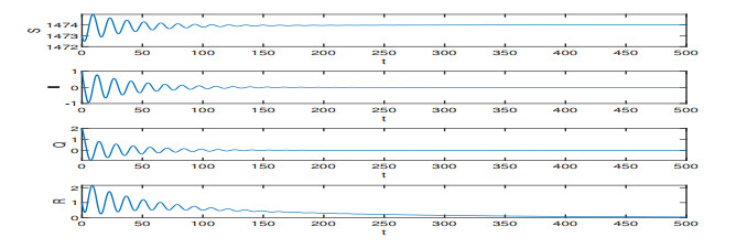
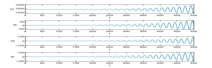
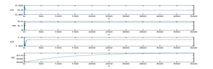
On the basis of the SIQR epidemic model, we consider the impact of treatment time on the epidemic situation, and we present a differential equation model with time-delay according to the characteristics of COVID-19. Firstly, we analyze the existence and stability of the equilibria in the modified COVID-19 epidemic model. Secondly, we analyze the existence of Hopf bifurcation, and derive the normal form of Hopf bifurcation by using the multiple time scales method. Then, we determine the direction of Hopf bifurcation and the stability of bifurcating periodic solutions. Finally, we carry out numerical simulations to verify the correctness of theoretical analysis with actual parameters, and show conclusions associated with the critical treatment time and the effect on epidemic for treatment time.

Keywords:

Citation: Hongfan Lu, Yuting Ding, Silin Gong, Shishi Wang. Mathematical modeling and dynamic analysis of SIQR model with delay for pandemic COVID-19[J]. Mathematical Biosciences and Engineering, 2021, 18(4): 3197-3214. doi: 10.3934/mbe.2021159

Related Papers:

[1]	Yurong Guan, Muhammad Aamir, Ziaur Rahman, Ammara Ali, Waheed Ahmed Abro, Zaheer Ahmed Dayo, Muhammad Shoaib Bhutta, Zhihua Hu . A framework for efficient brain tumor classification using MRI images. Mathematical Biosciences and Engineering, 2021, 18(5): 5790-5815. doi: 10.3934/mbe.2021292
[2]	Xiaobo Zhang, Donghai Zhai, Yan Yang, Yiling Zhang, Chunlin Wang . A novel semi-supervised multi-view clustering framework for screening Parkinson's disease. Mathematical Biosciences and Engineering, 2020, 17(4): 3395-3411. doi: 10.3934/mbe.2020192
[3]	Bakhtyar Ahmed Mohammed, Muzhir Shaban Al-Ani . An efficient approach to diagnose brain tumors through deep CNN. Mathematical Biosciences and Engineering, 2021, 18(1): 851-867. doi: 10.3934/mbe.2021045
[4]	Xiao Wang, Jianbiao Zhang, Ai Zhang, Jinchang Ren . TKRD: Trusted kernel rootkit detection for cybersecurity of VMs based on machine learning and memory forensic analysis. Mathematical Biosciences and Engineering, 2019, 16(4): 2650-2667. doi: 10.3934/mbe.2019132
[5]	Yufeng Qian . Exploration of machine algorithms based on deep learning model and feature extraction. Mathematical Biosciences and Engineering, 2021, 18(6): 7602-7618. doi: 10.3934/mbe.2021376
[6]	Tan Gao, Lan Zhao, Xudong Li, Wen Chen . Malware detection based on semi-supervised learning with malware visualization. Mathematical Biosciences and Engineering, 2021, 18(5): 5995-6011. doi: 10.3934/mbe.2021300
[7]	Jingren Niu, Qing Tan, Xiufen Zou, Suoqin Jin . Accurate prediction of glioma grades from radiomics using a multi-filter and multi-objective-based method. Mathematical Biosciences and Engineering, 2023, 20(2): 2890-2907. doi: 10.3934/mbe.2023136
[8]	Jian-xue Tian, Jue Zhang . Breast cancer diagnosis using feature extraction and boosted C5.0 decision tree algorithm with penalty factor. Mathematical Biosciences and Engineering, 2022, 19(3): 2193-2205. doi: 10.3934/mbe.2022102
[9]	Haifeng Song, Weiwei Yang, Songsong Dai, Haiyan Yuan . Multi-source remote sensing image classification based on two-channel densely connected convolutional networks. Mathematical Biosciences and Engineering, 2020, 17(6): 7353-7377. doi: 10.3934/mbe.2020376
[10]	Keyue Yan, Tengyue Li, João Alexandre Lobo Marques, Juntao Gao, Simon James Fong . A review on multimodal machine learning in medical diagnostics. Mathematical Biosciences and Engineering, 2023, 20(5): 8708-8726. doi: 10.3934/mbe.2023382

Abstract

1. Introduction

A brain tumor is comprised of abnormal cells in central spinal canal or brain or intracranial hard neoplasms, which are either benign or malignant ^[1]. In 2019 in the United States ^[2], about 86,010 new cases of non-malignant and malignant brain tumor are estimated to be analyzed. There were 79,718 deaths recognized to malignant brain between 2012 and 2016 with annual average mortality rate of 4.42. The mortality rate in adults and childern due to brain tumor has increased.

The brain tumor subtypes classification is challenging based on several factors. The experts still facing challenging to improve the detection accuracy by developing the latest technology. Several approaches are required to identify the brain tumor. The brain tumor is one of the fatal forms of cancer among other cancer types having agammaessive nature, heterogenous characteristics, and low survival rate. Due to several factors such as type, location and texture properties, the brain tumor is categorized into different types (e.g. Meningioma, CNS Lymphoma, Glioma, Acoustic Neuroma, Pituitary etc.) ^[3]. The clinically rate of incident of meningioma, pituitary, and glioma among other brain tumor types is 15%, 15% and 45% respectively ^[4]. The patient survival can be predicted and diagnosed based on the tumor type through which they can decide the relevant treatment choice ranging from chemotherapy to radiotherapy. Thus in order to properly planning and monitoring the brain tumor, tumor grading is highly desired ^[5].

The glioma is the major tumor type which has further three types such as 1) Ependymomas, 2) Astrocytomas, and 3) Oligodendrogliomas. From the glial cells, it originates and surround nerve cells. According to the genetic features, it can be further identified which help the prediction of future treatment and behavior. The meningioma is another type of tumor, which originates in brain. It occur in women and grow slowly without any symptom ^[6]. The pituitary tumor type grows in the pituitary gland. The pituitary glands are benign and don't spread in the whole body ^[6].

The researchers recently employed many artificial intelligences-based machine learning methods to predict the tumor. The feature extraction is the most crucial part in the machine learning techniques for computing the most relevant features, which is still a challenging task for researchers. In order to the select and compute the most relevant feature is a tedious task, which require the prior knowledge about the domain of the problem. The morphological features to detect the brain tumor types can led easily to misclassification as different tumor types have similar resemblance. The extracted features are then fed as input to the different brain tumor type ^[7]. Recently, the researchers have computed different feature extraction methods including Elliptic Fourier descriptors (EFDs), texture, scale invariant Fourier transform (SIFT) and morphological features. Rathore et al. ^[8] used ensemble methods to detect the colon biopsy by computing hybrid features. Rathore et al. ^[9] also computed geometric features for prediction of colon cancer. Hussain et al. ^[10] extracted EFDs, SIFT, texture, entropy and morphological features to detect the prostate cancer. Moreover, Asim et al. ^[11] computed the hybrid features to detect the Alzheimer disease (AD). The graphical method is expensive, and computer aided diagnosis (CAD) methods could not properly capture the background knowledge regarding the morphological features as these methods are based merely on the texture properties. To properly detect the brain tumor with its location, the radiologists analyzed the image features which are dependent on their personal skills and expertise. The hand-crafted features are still a tedious and challenging task as selecting and computing more relevant features is still challenging.

In the past, researchers employed various machine learning (ML) algorithms by computing various features extracting approaches in the medical fields. The Gray level co-occurrence matrix (GLCM) and Berkeley wavelet transform (BWT) features were extracted by ^[12] to detect brain tumor. Moreover, Reboucas et al. ^[13] computed GLCM features to analyze the human tissue densities. Dhruv et al. ^[14] studied the GLCM and Haralick texture features for the analysis of 3D medical images. Hussain et al. ^[10] applied support vector machines (SVM) with its kernels to detect prostate cancer by extracting combination of feature extracting strategies. Zheng et al. ^[15] integrated the SVM and graph cuts for medical image segmentation. Taie and Ghonaim ^[16] applied Chicken Swarm Optimization (CSO) based algorithms alongwith SVM for brain tumor's disease diagnosis. Abd-Ellah et al. ^[17] used kernel SVM to classify the brain tumor MRIs. Alquran et al. ^[18] applied SVM to detect the melanoma skin cancer. Wang et al. ^[19] proposed stationary wavelet entropy (SWE) to extract brain image features. They obtained improved classification performance results by replacing wavelet entropy (WE), discrete wavelet transform (DWT) and wavelet energy (WN) with the proposed SWE. The SWE averaged the variants of DWT. Zhang et al. ^[20] computed the Hu moment invariant (HMI) features from a specific MR brain image and then fed these HMI features to generalized eigenvalue proximal SVM (GEPSVM) and twin support vector machine (TSVM). The proposed methods outperformed in detection of brain tumor.

In this study, we extracted traditional features such as entropy, morphological, texture, EFDs, SIFT and proposed new feature extraction approach based on the RICA features to classify a multi-class brain tumor types and applied ML techniques.

The Figure 1 shows the schematic diagram to detect the Multi-class brain tumor types (i.e. Meningioma, Glioma and Pituitary) by extracting RICA based features from Brain MRIs and applied ML techniques such as SVM with its kernels and LDA with 10-fold cross validation. After extracting the features, the MRI data was split into 70% for training and 30% for testing.

Figure 1. Schematic Diagram to detect Multi-class Brain tumor types by computing RICA features and employing Machine learning techniques.

DownLoad: Full-Size Img PowerPoint

2. Material and methods

2.1. Dataset

The brain tumor CE-MRI dataset used in this study were taken from the publicly available database provided by the School of Biomedical Engineering, Southern Medical University, Guangzhou, China (https://figshare.com/articles/dataset/brain_tumor_dataset/1512427). The data details are used in the previous studies of detailed in ^[21] brain tumor adaptive sparse pooling, ^[22] brain tumor via region augmentation proposed by Cheng et al. ^[21,22] which contains 3064 T1-weighted contrast-enhanced MRI images acquired from Nanfang Hospital and General Hospital, Tianjin Medical University, China from 2005. There are three types of brain tumor from 233 patients including glioma (1426 slices), meningioma (708 slices) and pituitary (930 slices). All images were acquired from 233 patients in three planes: axial (994 images), sagittal (1025 images) and coronal (1045) image plane. The data is labelled as meningioma with 1, glioma with 2 and pituitary tumor with 3. In MR images, the experienced radiologists have designated the suspicious regions of interest (ROIs). The dataset was originally provided in matlab. mat format where each file stores a struct with a label which specify the type of tumor for a particular patient ID, brain image, image data in 512 × 512 unit 16 formats, vector storing the coordinates of the discrete points on tumor border, and a binary mask image with 1 indicating the tumor region. The images have an in-plane resolution of 512 × 512 with pixel size 0.49 × 0.49 mm². The thickness of slice is 6mm and gap of the slice is 1mm. Each patient contains approximately 1–6 images where most of patients have 1-3 images and very few patients have 4–6 images. The detail of CE-MRI data partitioning is detailed in section 2.4 and Table 1 below:

Table 1. Details of the CE-MRI dataset.

Tumor type	Number of Patients	Number of MR images	MRI view	Number of MR images
Meningioma	82	708	Axial Coronal Sagittal	209 268 231
Glioma	89	1426	Axial Coronal Sagittal	494 437 495
Pituitary	62	930	Axial Coronal Sagittal	291 319 320
Total	233	3064		3064

| Show Table

DownLoad: CSV

In this study, we divided data into train and test based on patient-ID, where 70% of patients data was used for training and 30% for testing purpose for tumor type based on single slice assigned to each tumor type as performed in the previous studies Cheng et al. Abiwinanda et. al.^[23], Cheng et al. ^[22], Sajjad et al. ^[24], Zia et al. ^[25], Badža and Barjaktarović ^[26], Gumaei et al. ^[27], Swati et al. ^[4], and Huang et al. ^[28]. In order to overcome the problem of overfitting, 10-fold cross-validation was also performed.

2.2. Feature extraction

For improving the detection performance, the extraction of most relevant features is one of the most important steps. We extracting hybrid features as employed in our recent studies such as to detect prostate cancer by extracting combination of features ^[10], congestive heart failure with multimodal features ^[29], arrhythmia detection with hybrid features ^[30] proposed by Hussain et al. ^[10,29,30]. In this study, we computed traditional features based on morphological features and texture features, alongwith robust RICA features from multi-class brain tumor (pituitary, glioma and meningioma) and applied ML methods including SVM with its kernels and LDA. The RICA features based on their sparsity and robust to noise is more robust, and sigmoid nonlinearity imaging data. The brain tumor types are categorized into several factors such as type, location, texture of tumor. Thus, the traditional features may not provide detection performance better. On contrast, the RICA features seemed to be more appropriate to compute the multivariate information hidden in the brain tumor types. The traditional features extracted were of following categories:

2.2.1. Texture features

Texture feature have effectively utilized in solving classification related issue ^[31] especially to classify colon biopsies by employing microscopic image analysis for feature identification ^[32], Fractal analysis ^[33] proposed by Esgiar et al. ^[32,33]. Texture features are obtained from Gray-level co-occurrence matrix (GLCM). GLCM covers the spatial relationship of the Gray-level in an image. Any entry (i, j) th in co- occurrence matrix explain the occurrence of Gray-level i and j, their relative orientation ʘ and their distance d. Commonly ʘ correspond in four direction (0⁰, 45⁰, 90⁰, 135⁰⁾. There are around 15 feature which obtained using GLCM which we studied as Angular second moment, Entropy, Correlation, Local Homogeneity, Shade, Variance, Average, Sum, Prominence, Difference Entropy, Sum Entropy, Difference variance Contrast, Sum variance and Information measure of correlation. The texture features extracted from brain tumor types are reflected in Table 2 below.

Table 2. Texture Features.

Features	Formulas	Description
Contrast (t)	$\sum\limits_{x=1}^{K}\sum\limits_{y=1}^{K}{(x-y)}^{2}{p}_{xy}$	It is used to measure the contract between current pixel and its neighbor.
Correlation (ρ)	$\sum\limits_{x=1}^{K}\sum\limits_{y=1}^{K}\frac{(x-{\mu }_{x})(y-{\mu }_{y}){p}_{xy}}{{\sigma }_{x}{\sigma }_{y}}$	It is used to measure the degree of correlation between current pixel and its neighbor.
Dissimilarity (Dis)	$\sum\limits_{x=1}^{K}\sum\limits_{y=1}^{K}\left\|x-y\right\|{p}_{xy}$	It is used to measure the difference in images.
Entropy	$\sum\limits_{x=1}^{K}\sum\limits_{y=1}^{K}{p}_{xy}(-ln{p}_{xy})$	It is used to get the encoded information from an image.
Energy (n)	$\sum\limits_{x=1}^{K}\sum\limits_{y=1}^{K}{p}_{{xy}^{2}}$	It is used to measure the uniformity of an image.
Homogeneity (h)	$\sum\limits_{x=1}^{K}\sum\limits_{y=1}^{K}\frac{{p}_{xy}}{1+\|x-y\|}$	It is used to calculate the spatial closeness of elements in G to the diagonal of the matrix.
Randomness (r)	$-\sum\limits_{x=1}^{K}\sum\limits_{y=1}^{K}{p}_{xy}{log}_{2}{p}_{xy}$	It is used to measure the randomness of the elements of the GLCM.
Mean (µ)	${\mu }_{x}=\sum\limits_{x=1}^{K}\sum\limits_{y=1}^{K}x({p}_{xy})$ ${\mu }_{y}=\sum\limits_{x=1}^{K}\sum\limits_{y=1}^{K}y({p}_{xy})$	This formula is used to calculate the sum of all values and P is the probability mass function.
Variance (σ²)	${\sigma }_{x}^{2}=\sum\limits_{x=1}^{K}\sum\limits_{y=1}^{K}({p}_{xy}\left)\right(x-{\mu }_{x}{)}^{2}$ ${\sigma }_{y}^{2}=\sum\limits_{x=1}^{K}\sum\limits_{y=1}^{K}({p}_{xy}\left)\right(y-{\mu }_{y}{)}^{2}$	This equation is used to measure how far a set of numbers is spread out from their mean.
Standard Deviation (σ)	${\sigma }_{x}$ = $\sqrt{{\sigma }_{x}^{2}}$ & ${\sigma }_{y}$ = $\sqrt{{\sigma }_{y}^{2}}$	It is used to quantify the amount of dispersion of different values of a data set.

| Show Table

DownLoad: CSV

These features can be computed from GLCM matrix G, where x and y represent indices of rows and columns of matrix G. ${p}_{xy}$ is the ${xy}^{th}$ term of matrix G divided by the sum of elements. The term ${\mu }_{x}$ and ${\mu }_{y}$ are the mean, ${\sigma }_{x}$ and ${\sigma }_{y}$ are the standard deviation of xth row and yth column of matrix G.

2.2.2. Morphological features

Morphology of skins plays vital part in deciding either the tissues are malignant or oppositely normal. Morphological features give an approach to change over the image morphology values. These features are obtained from images through changing the morphology of image within set of quantitative values utilizes in classification and they have extensively been utilized as a part of classification ^[34] segmentation ^[35]. Morphological feature module (FEM) taking input in form of the binary batch also finds associated factors in the clusters. Researchers in the past extracted few morphological features such as Perimeter (p), Eccentricity (y), Area (a), Convex Area (x), Euler Number (l), Orientation (e), Compactness (0), Length of major (m1), and Minor Axes (m2) etc. In this study, we computed the following morphological features as reflected in Table 3:

Table 3. Morphological Features.

Features	Formulas	Description
Area (A)	Total number of pixels in a region	Total count of pixels that a specific region of image contains
Perimeter (P)	Pixels at the boundary of an image	Total count of pixels at the boundary of the image
Solidity	$\frac{\mathrm{A}\mathrm{r}\mathrm{e}\mathrm{a}}{\mathrm{C}\mathrm{o}\mathrm{n}\mathrm{v}\mathrm{e}\mathrm{x}\mathrm{A}\mathrm{r}\mathrm{e}\mathrm{a}}$	To calculate the density of an object, ratio between area and full convex object.
Roundness	$\frac{4\mathrm{ }\times \mathrm{\Pi }\times \mathrm{A}\mathrm{r}\mathrm{e}\mathrm{a}}{{\left(\mathrm{C}\mathrm{o}\mathrm{n}\mathrm{v}\mathrm{e}\mathrm{x}\mathrm{P}\mathrm{e}\mathrm{r}\mathrm{i}\mathrm{m}\mathrm{e}\mathrm{t}\mathrm{e}\mathrm{r}\right)}^{2}}$	This equation is used to illustrate the difference between line and circle from other region of image.
Convex Area	Total no of pixels in a convex image	It is used to count total no of pixels in convex image.
Convexity	$\frac{\mathrm{C}\mathrm{o}\mathrm{n}\mathrm{v}\mathrm{e}\mathrm{x}\mathrm{P}\mathrm{e}\mathrm{r}\mathrm{i}\mathrm{m}\mathrm{e}\mathrm{t}\mathrm{e}\mathrm{r}}{\mathrm{P}\mathrm{e}\mathrm{r}\mathrm{i}\mathrm{m}\mathrm{e}\mathrm{t}\mathrm{e}\mathrm{r}}$	This equation is used to calculate the perimeter ratio between object itself and convex full of object.
Compactness	$\frac{4\mathrm{ }\times \mathrm{\Pi }\times \mathrm{A}\mathrm{r}\mathrm{e}\mathrm{a}}{{\left(\mathrm{P}\mathrm{e}\mathrm{r}\mathrm{i}\mathrm{m}\mathrm{e}\mathrm{t}\mathrm{e}\mathrm{r}\right)}^{2}}$	It is used to find the degree of deviation from a circle. This shows the ratio between the object areas with circle area.
Maximum Radius (Max_R)	MAX(DISTANCE(C(x, y), BOUNDARY(x, y)))	This formula is used to calculate the maximum distance from boundary of the image to the center of the image, x and y are two points on the image.
Minimum Radius (MIN_R)	MIN(DISTANCE(C(x, y), BOUNDARY(x, y)))	This formula is used to calculate the minimum distance from boundary of the image to the center of the image.
Euler Number (EUL_NO)	No of objects in region – No of holes in these objects	This formula provides the difference between effected and unaffected area of an image.
Standard Deviation	$\sqrt{\frac{1}{\mathrm{n}}\sum \limits_{\mathrm{i}=1}^{\mathrm{n}}{\left({\mathrm{x}}_{\mathrm{i}}-\stackrel{-}{\mathrm{x}}\right)}^{2}}$	It is used to calculate the contrast of an image.
Entropy	$\sum {\left(\mathrm{p}\mathrm{*}{\mathrm{l}\mathrm{o}\mathrm{g}}_{2}\left(\mathrm{p}\right)\right)}^{2}$	This equation shows the statistical measure which can be used to get the texture of the image.
Eccentricity (ECT)	$\sqrt{\left(\frac{{\mathrm{M}\mathrm{A}\mathrm{X}}_{\mathrm{R}}-{\mathrm{M}\mathrm{I}\mathrm{N}}_{\mathrm{R}}}{{\mathrm{M}\mathrm{A}\mathrm{X}}_{\mathrm{R}}}\right)^{2}}$	This formula represents the ratio of distance between major axis and ellipse focal. Value can be 0-1.
Rectangularity	$\frac{\mathrm{A}\mathrm{r}\mathrm{e}\mathrm{a}}{{\mathrm{M}\mathrm{A}\mathrm{X}}_{\mathrm{R}}-{\mathrm{M}\mathrm{I}\mathrm{N}}_{\mathrm{R}}}$	This formula is used to identify the similarity of image shape with rectangular shape.
Elongation	1 $-\frac{{\mathrm{M}\mathrm{I}\mathrm{N}}_{\mathrm{R}}}{{\mathrm{M}\mathrm{A}\mathrm{X}}_{\mathrm{R}}}$	This formula is used to measure the length of the object.

| Show Table

DownLoad: CSV

2.2.3. Reconstruction Independent Component Analysis (RICA)

The RICA does not require any class label information because of its un-supervised nature. The ICA algorithm deficiencies were removed using RICA algorithm. The results yielded using RICA are more robust than ICA. This algorithm learns based on the sparse feature learning mechanism. The algorithm based on the sparse filter is capable to distinguish the various made natural signals, and these features can play a vital role in many of the ML techniques.

Consider an unlabeled data with input ${\{y}^{\left(i\right)}{\}}_{i = 1}^{n}, {y}^{\left(i\right)}\in {\mathbb{R}}^{m},$ the optimization problem of standard ICA using optimization algorithms ^[36], kernel sparse representation ^[37] for estimating ICA ^[36,37] mathematically defied as:

$_X^{min}\frac{1}{n}\sum _{i = 1}^{n}h\left(X{y}^{i}\right)$

(2.1)

$Subject \;to\dots {XX}^{U} = I$

Where h(.) indicate nonlinear penalty function, $X\in {S}^{Lxm}$ is a matrix, L represent number of vectors and I is the identity matrix. Additionally, ${XX}^{U} = I$ is used for avoiding the vectors in X to become degenerate. A smooth penalty function is used to handle this situation as indicated below:

$h(.) = log (cosh (.)[38].$

(2.2)

To completely learn the standard ICA, there are several orthonormality constraint which obstruct it. Subsequently, this drawback stops ICA from scaling to high dimensional data. To resolve this matter, the soft reconstruction cost is used in RICA. Thus, RICA after this replacement, can be characterized by following equation (2.3)

$_X^{min}\frac{\lambda}{n}\sum _{i = 1}^{n}\left(\left|\right|{X}^{U}X{y}^{i}-{y}^{i}{\left|\right|}_{2}^{2}+\sum _{i = 1}^{n}\sum _{k = 1}^{l}h\left({X}_{k}{y}^{i}\right)\right)$

(2.3)

Here parameter λ > 0 shows the tradeoff between reconstruction error and sparsity.

The penalty h can produce sparse representations only, but not invariant ^[38]. Thus, RICA using efficient overcomplete feature learning algorithms ^[39], building low level features using feature learning ^[40] studied by V Le et al. ^[39,40] swapped it by an extra L₂ pooling penalty, by promoting pooling features to cluster correlated features together. Furthermore, feature learning can be done using L₂ pooling. L₂ pooling using feature pooling ^[41], learning invariant features ^[42] studied by ^[41,42] is a two-layered network having square nonlinearity in the 1^st layer ${\left(.\right)}^{2}$ and square root nonlinearity in the 2^nd layer $\sqrt{(.)}$ as reflected in equation (2.4)

$h\left(X{y}^{i}\right) = \sum _{k = 1}^{L}\sqrt{\varepsilon +{H}_{k}.\left(\left(X{y}^{i}\right)\odot\left(X{y}^{i}\right)\right)}$

(2.4)

Here ${H}_{k}$ represents a row of spatial pooling matrix H $\in {P}^{L\times L}$ set to constant weights i.e., 1 for each element in matrix H, $\odot$ represents the element wise multiplication and ε > 0 is a small constant.

The sparse representation of the actual data can be represented using RICA. The following steps are used to compute the RICA features.

The step-by-step procedure to compute the features using RICA algorithm is reflected in the Figure 2. The RICA feature model is obtained by applying RICA to the matrix of predictor data X containing p variables q number of features to extract from X. The RICA thus learns p by q matrix of transformation weights. The value of q can be less than or greater than the number of predictor variables to avoid from undercomplete or overcomplete feature representation. In this study, we choose q to 100 features and default values of alpha and gamma are set.

Figure 2. Steps in computing features based on RICA Algorithm.

DownLoad: Full-Size Img PowerPoint

2.3. Classification methods

2.3.1. Support Vector Machine (SVM)

Vladimir Vapnik proposed SVM in 1979, which is a state of art algorithm used in different fields including medical diagnosis area ^[43], visual pattern recognition ^[44] and machine learning ^[45]. SVM is successfully used in many applications including text recognition, face expression recognition, emotion recognition, biometrics, and content-based image retrial etc. It constructs a hyperplane in the infinite dimensional space. The hyperplane helps to achieve the largest distance to any nearest training data point of any class. The lower generalization error can be obtained with the larger functional margin. To achieve this, SVM use the kernel trick. The linear and nonlinear separation with margin and slack variables in case of error examples are reflected in the Figure 3 (a, b) and Figure 4 (a, b).

Figure 3. SVM (a) linear separation and (b) Margin.

DownLoad: Full-Size Img PowerPoint

Figure 4. (a) Error on margin using slack variable, (b, c) SVM non-linear separation.

DownLoad: Full-Size Img PowerPoint

Consider a hyperplane defined by x.w + b = 0, where w is its normal. The data is linearly separated and is labelled as:

$\left\{{x}_{i}, {y}_{i}\right\}, {x}_{i}ϵ{R}^{N}d, {y}_{i}ϵ\left\{-1, 1\right\}, i = 1, 2, \dots \dots , N$

(2.5)

Here ${y}_{i}$ is the class label of two class SVM. To obtain the optimal boundary, the objective function is minimized with maximal margin i.e. $E = {‖w‖}^{2}$ subject to

${x}_{i}.w+b\ge 1\;for\;{y}_{i} = +1$

${x}_{i}.w+b\le 1 \;for\;{y}_{i} = -1$

(2.6)

Combining these into set of inequalities as

${(x}_{i}.b+b){y}_{i}\ge 1\;for\;all\;i$

Generally, the data is not linearly separable, in such cases a slack variable ${\mathrm{\Xi }}_{i}$ is used to indicate the amount of misclassification rate. Thus, new subjective function is then reformulated as:

$E = \frac{1}{2}{‖w‖}^{2}+C\sum \limits_{i}L\left({\mathrm{\Xi }}_{i}\right)$

(2.7)

Subject to

${(x}_{i}.b+b){y}_{i}\ge 1-{\xi }_{i}\;for\;all\;i$

The first term on the right-hand side is the regularization term which gives the SVM an ability to generalize the sparse data well. The points which lie outside the margin are represented by the second term denoted by the empirical risk. The cost function is denoted by L, and hyper parameter is denoted by C, which shows a trade-off effect by minimizing the empirical risk against maximizing the margin. Linear-error cost function is most used because of its ability to detect the outliers. The dual formulation with

$L\left({\mathrm{\Xi }}_{i}\right) = {\mathrm{\Xi }}_{i}\;is$

${\alpha }^{*} = {max}_{\alpha }\left(\sum\limits_{i}{\alpha }_{i}+\sum\limits_{i, j}{\alpha }_{i}{\alpha }_{j}{y}_{i}{y}_{j}{x}_{i}{x}_{j}\right)$

(2.8)

Subject to

$0\le {\alpha }_{i}\le C\;and\;\sum\limits_{i}{\alpha }_{i}{y}_{j} = 0$

In which $\alpha = \left\{{\alpha }_{1}, {\alpha }_{2}, {\alpha }_{3}, ......{\alpha }_{i}, \right\}$ is a set of Lagrange multipliers of the constraints in the primal optimization problem. The optimal decision boundary is now given by.

${w}_{0} = \sum\limits_{i}{\alpha }_{i}{x}_{i}{y}_{i}$

(2.9)

SVM for non-linearly separable data

The kernel function trick is recommended by the Muller et al. (2001) to deal the data with nonlinear separability. In this case the non-linear mapping from input space is made to higher dimensional feature space. The dot product between two vectors in the input space is expressed by dot product with some kernel functions in the feature space.

The Figure 5 reflects the SVM kernels parameter optimization settings. The kernel parameters, box constraints, polynomial order (1, 2, 3) were used according to the default settings. As shown in the above figure, in this research work three SVM kernels (Linear, Quadratic, cubic) are used for the classification of Brain Tumor. All three SVM classifiers are trained with 10-Fold Cross-validation and Kernel Scale auto. Box Constant parameter is used to control the overfitting problem. SVM is a binary classifier and to train on multi-class, Coding parameter oneVSone is used. In the oneVSone option, one class is treated as a positive, the other as a negative class, and all other classes are not used in training, this process repeated for all the class combinations.

Figure 5. Parameter optimizations for SVM kernels.

DownLoad: Full-Size Img PowerPoint

The most used kernel functions are polynomial and radial base function (RBF). Mathematically, these are expressed as:

Types of Different Machine Learning Kernels with formulae

SVM Linear Kernel

$K\left({x}_{i}, {y}_{i}\right) = {x}_{i}.{y}_{i}+1$

(2.10)

SVM Quadratic Kernel

$K\left({x}_{i}, {y}_{i}\right) = ({x}_{i}.{y}_{i}+1{)}^{2}$

(2.11)

SVM Cubic Kernel

$K\left({x}_{i}, {y}_{i}\right) = ({x}_{i}.{y}_{i}+1{)}^{3}$

(2.12)

2.3.2. Linear Discriminant Analysis (LDA)

Belhumeur in 1997 ^[46] proposed LDA as one of the classical algorithms in the field of pattern recognition and artificial intelligence (AI). The main functionality of this algorithm is to project the high dimensional samples into low dimensional space to achieve the effect of extracting classification information and to compress the feature space dimension. LDA is successfully been employed in many of the applications such as Pathak et al. ^[47] applied this algorithm for removing the redundancy and inconsistency in the data. Moreover, LDA can be used for classification and dimensionality reduction, we used LDA for multi-class classification.

LDA is a simple method of classification using the generative methodology. It assumes that a Gaussian distribution is possible for each class and that every class has the same matrix of covariance. The LDA is a linear classification method with these assumptions. If they are by chance supportive of the actual data distribution, LDA is optimal in that it converges to the classifier of Bayes, when the number of data tends to infinitely (the parameter estimates, therefore, correspond to the real distribution parameters). In fact, LDA needs few computations to approximate the parameters of the classifier that amount to the estimation of the percentages and means plus the inversion of the matrix.). The LDA takes the generative method when presuming that a Gaussian distribution with probability density function generates the data of each class. The probability density function of $x$ in population ${\pi }_{i}$ is multivariate natural with mean variable ${\mu }_{i}$ and variance-covariance matrix. The formula for this usual function of probability density is:

${p}_{X|Y = y}\left(\boldsymbol{x}\right|Y = y) = \frac{1}{\left(2\pi {)}^{\frac{d}{2}}\right|{\bf{\Sigma }}_{y}{|}^{\frac{1}{2}}}\mathrm{e}\mathrm{x}\mathrm{p}(-\frac{1}{2}\left(\boldsymbol{x}-{\boldsymbol{\mu }}_{y}{)}^{T}{\bf{\Sigma }}_{y}^{-1}\left(\boldsymbol{x}-{\boldsymbol{\mu }}_{y}\right)\right)$

(2.13)

And that the covariance matrix ${\bf{\Sigma }}_{y}$ for all labels is the same:

$\forall y\in \mathcal{Y}, {\bf{\Sigma }}_{y} = \bf{\Sigma }$

(2.14)

They approximate the parameters as follows. The previous probabilities are essentially the data point fractions of each group:

$\forall y\in \mathcal{Y}, P(Y = y) = \frac{{N}_{y}}{N}, \text{with}\;{N}_{y} = \sum\limits_{i = 1}^{N}{\bf 1}_{{y}_{i} = y}$

(2.15)

The Gaussians' means are estimated by the means of the sample.

$\forall y\in \mathcal{Y}, {\boldsymbol{\mu }}_{k} = \frac{1}{{N}_{y}}\sum\limits_{{y}_{i} = y}{\boldsymbol{x}}_{i}$

(2.16)

And the matrix for covariance by

${\bf{\Sigma }} = \frac{1}{N-\left|\mathcal{Y}\right|}\sum\limits_{y\in \mathcal{Y}}.\sum\limits_{{y}_{i} = y}({\boldsymbol{x}}_{i}-{\boldsymbol{\mu }}_{y})({\boldsymbol{x}}_{i}-{\boldsymbol{\mu }}_{y}{)}^{T}$

(2.17)

2.4. Training/Testing Data Formulation

For training/testing data formulation, the Jack-knife 10-fold cross validation (CV) was used. The performance was evaluated using the similar metrics to detect brain tumor by applying adaptive spatial pooling methods ^[21], margin information and learning distance metric ^[48], bag-of-visual word representation methods ^[49], spatial layout information based methods ^[50] as employed and tested by ^{[21,48,49,50]}, and CE-MRI data of 233 patients was randomly divided into 10 subsets of equal size. We also ensured that there is no overlap and equal ratios of the different type of tumors in the 10 subsets for the CE-MRI datasets. The division according to the patients ensure that images from same patient did not exist simultaneously in the training and testing set. Using 10-fold cross validation, the data is partitioned into 10 folds and 9 folds participate in training and remaining folds in testing. The samples in the test fold are purely unseen. The entire process is repeated 10 times.

K-fold Cross-validation is an effective preventative measure against overfitting. Thus, to tune the model, the dataset is split into multiple train-test bins. Using k-fold CV, the dataset is divided into k-folds. For model training, k-1 folds are involved, and rest of the folds are used for model testing. Moreover, k-fold method is helpful for fine-tuning the hyperparameters with the given original training dataset in order to determine that how the outcome of ML model could be generalized. The k-fold cross validation procedure is reflected in Figure 6 below.

Figure 6. K-fold Cross-validation.

DownLoad: Full-Size Img PowerPoint

3. Results and discussions

The researchers are devising automated tools to improve the prediction of brain tumor types because of the multivariate characteristics of the tumor types. Extracting the most relevant and appropriate feature is still a challenging task. In this study, we first extracted the traditional texture and morphological features from brain tumor types and computed the performance using the machine learning classification techniques such as LDA, SVM with linear, quadratic, cubic and cosine kernels. We then extracted the RICA based features based on the multivariate characteristics. These features are then used as input to these classifiers for multi-class approach. The results reveal that proposed feature extraction approach using SVM cubic yielded more appropriate results to predict the tumor types.

Table 4 shows the results of AI multiclass brain tumor types (Glioma, meningioma, pituitary) classification of texture and morphological features. The classifiers LDA and SVM with its kernel yielded moderate performance. Specifically, SVM quadratic classifiers yielded best performance with accuracy (93.11%), AUC (0.8928) followed by SVM cubic with accuracy (93.04%) and AUC (0.8895) to predict the pituitary from multiclass. The other performance metrics are reflected in the Table 3.

Table 4. Multiclass classification of Brain tumor types (Glioma, meningioma, pituitary) by extracting texture + morphological based features and employing machine learning techniques.

Class	Sens.	Spec.	PPV	NPV	FPR	Acc.	AUC
LDA
Glioma	100%	16.09%	47.79%	100%	0.839	52.54%	0.5804
meningioma		100%		100%	0	100%
Pituitary	39.78%	100%	100%	94.31%	0	94.52%	0.6989
SVM Linear
Glioma	100%	54.42%	60.67%	100%	0.455	73.24%	0.7720
meningioma		100%		100%	0	100%
Pituitary	75.48%	100%	100%	89.67%	0	92.16%	0.8774
SVM Quadratic
Glioma	100%	62.30%	63.95%	100%	0.376	77.42%	0.8115
meningioma	52.28%	99.79%	93.02%	97.54%	0.0020	97.42%	0.7604
Pituitary	78.57%	100%	100%	90.78%	0	93.11%	0.8928
SVM Cubic
Glioma	100%	71.25%	64.91%	100%	0.2875	81.23%	0.8562
meningioma	46.80%	98.56%	83.89%	92.04%	0.014	91.41%	0.7268
Pituitary	77.90%	100%	100%	90.79%	0	93.04%	0.8895
SVM Cosine
Glioma	100%	75.50%	67.42%	100%	0.2449	83.74%	0.8775
meningioma	47.61%	99.29%	90.45%	93.08%	0.007	92.92%	0.7345
Pituitary	71.79%	100%	100%	85.71%	0	89.95%	0.8589

| Show Table

DownLoad: CSV

Table 5 reflect the multi-class classification results of brain tumor types (meningioma, Glioma, pituitary) based on the RICA features. The classifiers LDA and SVM with its kernel yielded highest performance. Specifically, SVM cubic classifiers yielded best performance with accuracy (99.34%), AUC (0.9892) followed by SVM quadratic with accuracy (98.10%) and AUC (0.9699) to predict the pituitary from multiclass. To predict the meningioma from multiclass, SVM cubic yielded an accuracy (96.96%), AUC (0.9348) and to predict glioma from multiclass and accuracy (95.88%), AUC (0.9635) was obtained. The highest multi-class prediction with other classifiers was obtained by LDA followed by SVM linear, and SVM cosine.

Table 5. Multiclass classification of Brain tumor types by extracting RICA based features and utilizing ML techniques.

Class	Sensitivity	Specificity	PPV	NPV	FPR	Accuracy	AUC
LDA
Glioma	100%	82.38%	78.95%	100%	0.1761	89.39%	0.9119
meningioma	69.18%	99.32%	95.66%	93.75%	0.0067	93.99%	0.8425
Pituitary	89.07	100%	100%	95.24%	0	96.57%	0.9453
SVM Linear
Glioma	100%	84.64%	81.45%	100%	0.153	90.83%	0.9232
meningioma	71.50%	99.60%	97.46%	94.26%	0.004	94.68%	0.8555
Pituitary	88.32%	100%	100%	94.63%	0	96.18%	0.9416
SVM Quadratic
Glioma	100%	91.18%	89.53%	100%	0.088	94.97%	0.9559
meningioma	84.51%	99.63%	98.31%	96.20%	0.0036	96.57%	0.9207
Pituitary	93.89%	100%	100%	97.31%	0	98.10%	0.9699
SVM Cubic
Glioma	100%	92.27%	91.38%	100%	0.072	95.88%	0.9635
meningioma	87.34%	99.62%	98.47%	96.60%	0.0038	96.96%	0.9348
Pituitary	97.78%	100%	100%	99.07%	0	99.34%	0.9892
SVM Cosine
Glioma	100%	87.51%	84.01%	100%	0.1248	92.46%	0.9375
meningioma	72.98%	99.76%	98.66%	93.72%	0.0024	94.45%	0.8636
Pituitary	87.27%	100%	100%	94.14%	0	95.58%	0.9336

| Show Table

DownLoad: CSV

The Figure 7 (a–e) reflects the Multi-class distribution of glioma (1426 slices), meningioma (708 slices) and pituitary (930 slices). From figure 7 (d) using SVM cubic, out of 1426 glioma, there were 1337 were predicted a glioma, 113 as meningioma and 13 as pituitary. From 708 meningioma, after prediction, there were 84 predicted as glioma, 580 as meningioma and 9 as pituitary. From 930 pituitary, there were 5 predicted as glioma, 15 as meningioma and 908 as pituitary. The distribution using other classifiers is reflected in the Figure 7 (a–e).

Figure 7. Confusion matrix to detect Multi-class brain tumor types (Glioma, Pituitary, Meningioma) by Computing RICA features and using machine learning techniques a) LDA, b) SVM linear, c) SVM quadratic, d) SVM cubic, e) SVM cosine.

DownLoad: Full-Size Img PowerPoint

The researchers extracted various features extraction approaches using ML and DL methods to detect the binary class classification of brain tumor types. The highest performance based on the overall accuracy was obtained by ^[22] 91.28%, ^[51] 90.89%, ^[52] 86.56%, and ^[53] 84.19%. With the multi-class classification, the LDA yielded accuracy for pituitary (96.48%), meningioma (93.89%) and glioma (89.39%). Using SVM linear, the accuracy to detect pituitary was yielded (96.28%), an accuracy (94.45%) was obtained to detect meningioma, while to detect the glioma, and accuracy (90.76%) was yielded. By employing the quadratic kernel, the highest detection was obtained to detect pituitary with accuracy (98.07%), followed by accuracy (96.18%) to predict meningioma and accuracy (94.35%) to detect glioma.

The Figure 8 (a–c) shows the multi-class separation in the form of the area under the receiver operating curve based on texture + morphological features extracted and employing machine learning techniques. The highest separation was obtained with AUC (0.8928) to detect pituitary using SVM quadratic followed by AUC (0.8895) to detect pituitary using SVM cubic.

Figure 8. Area under the receiver operating curve (AUC) to detect Multi-class Brain tumor types a) Glioma, b) Meningioma, c) Pituitary using Robust Machine learning classifiers and extracting texture + morphological features.

DownLoad: Full-Size Img PowerPoint

The Figure 9 (a-c) reflect the Multi-class separation to distinguish a) Glioma, b) Meningioma, and c) Pituitary by computing RICA features and utilizing robust machine learning techniques. To detect the Glioma, the separation with AUC was obtained using LDA (0.9119), SVM Linear (0.9232), SVM quadratic (0.9559), SVM cubic (0.9635), and SVM cosine (0.9375). To detect the meningioma, the separation with AUC was obtained using LDA (0.8425), SVM Linear (0.8555), SVM quadratic (0.9207), SVM cubic (0.9348), and SVM cosine (0.8636). To detect the pituitary, the separation with AUC was obtained using LDA (0.9453), SVM Linear (0.9416), SVM quadratic (0.9699), SVM cubic (0.9892), and SVM cosine (0.9336).

Figure 9. Area under the receiver operating curve (AUC) to detect Multi-class Brain tumor types a) Glioma, b) Meningioma, c) Pituitary using Robust Machine learning classifiers by extracting RICA features.

DownLoad: Full-Size Img PowerPoint

The Table 6 presents the findings of different hand-crafted features techniques alongwith machine learning techniques to classify the brain tumor from normal and between brain tumor types using similar dataset and different datasets. Using LDA, the highest detection performance was obtained to detect pituitary with accuracy (96.57%), AUC (0.9453) followed by meningioma and glioma. Using SVM linear kernel, the highest detection performance was obtained to detect pituitary with accuracy (96.18%), AUC (0.9416). Using SVM quadratic kernel, the highest detection performance was obtained to detect pituitary with accuracy (98.10%) and AUC (0.9699). Likewise, using SVM cubic, the highest detection performance to detect the pituitary was obtained with accuracy (99.34%), AUC (0.9892). Moreover, using SVM cosine, to detect pituitary an accuracy (95.58%) and AUC (0.9336) was yielded.

To extract the diagnostic information from MR images, researchers employed several image analysis techniques using tissue characterization methods ^[57], texture text objects and intracranial brain tumor detection ^[58], and tissue characterization and intracranial brain tumor detection ^[59] detailed in ^[57,58,59]. The texture analysis and pattern recognition techniques were employed in these studies to characterize the types of brain tumor. Recently, ^[60] employed SVM to classify the gliomas and meningiomas and obtained 95% overall accuracy to distinguish these types. Moreover, ^[57] employed k-nearest neighbor and discriminant analysis to distinguish between oedematous and brain tumor tissues by achieving a maximum accuracy of 95%. Recently, several studies applied MR spectroscopic features such as long echo proton MRs signals ^[61], short echo time ^[62], tumor grading ^[63], short time multicenter study ^[64], and short echo metabolic patterns ^[65] as described in ^{[61,62,63,64,65]} or combination of spectroscopic and texture features to distinguish between various brain tumor types by achieving a maximum accuracy of 99% ^[64]. Moreover, authors with benchmark with similar dataset ^[37] extracted hand-crafted features by applying machine learning techniques and deep convolutional neural network methods obtained performance in terms of overall accuracy ^[7] 98%, ^[54] 96.4%, ^[66] 80%, ^[52] 86.56%, ^[25] 85.69%, ^[22] 91.28%, ^[55] 94.2%, ^[53] 91.43%, and ^[56] 96.67%. In the present study, we used MRI brain tumor types dataset originally provided by Cheng et al. which is used in his studies ^[21,22]. We compared the results with similar dataset used by other researchers such as Abiwinanda et. al. ^[23], Cheng et al. ^[22], Sajjad et al. ^[24], Zia et al. ^[25], Badža and Barjaktarović ^[26], Gumaei et al. ^[27], Swati et al. ^[4], and Huang et al. ^[28] as reflected in Table 6.

Table 6. Literature review of existing techniques and methods and with similar dataset.

Author	Feature/Methods	Performance
Machhale et al. ^[7]	SVM-KNN	Sensitivity: 100% Specificity: 93.75% Accuracy: 98%
Zacharaki et al. ^[54]	Cross-Validation Using different Classifiers (LDA, k-NN, SVM)	Sensitivity: 75% Specificity: 100% Accuracy: 96.4%
Badža and Barjaktarović ^[26]	CNN	Accuracy 95.40%
Gumaei et al. ^[27]	Regularized extreme learning machine (RELM)	Accuracy 94.23%
Swati et al. ^[4]	Automatic content-based image retrieval (CBIR) system	Average precision 96.13%
Huang et al. ^[28]	convolutional neural network based on complex networks (CNNBCN)	Accuracy 95.49%
Afshar et al. ^[52]	Capsule Network Method	Accuracy: 86.56%
Zia et al. ^[25]	Window Based Image Cropping	Sensitivity:86.26% Specificity:90.90% Accuracy: 85.69%
Sajjad et al. ^[24]	CNN with data augmentation	Sensitivity:88.41% Secificity:96.12% Accuracy: 94.58%
Cheng et al. ^[22]	Feature extraction methods: Intensity Histogram GLCM BOW Classification Methods: SVM SRC KNN	Accuracy:91.28%
Abiwinanda et. al. ^[23]	CNN	Accuracy: 84.19%
Anaraki et al. ^[55]	Genetic Algorithms	Accuracy: 94.2%
Paul et al. ^[53]	NN	Accuracy: 91.43%
Sachdeva et al. ^[56]	Segmentation and Feature extraction	Highest accuracy 96.67%
This work	RICA Based Features SVM Cubic with Multiclass classification 1) Pituitary 2) Meningioma 3) Glioma	1) Accuracy: 99.34%, AUC: 0.9892 2) Accuracy: 96.96%, AUC: 0.9348 3) Accuracy: 95.88%, AUC: 0.9635

| Show Table

DownLoad: CSV

The authors who used the similar database includes Abiwinanda et. al., Sajjad et al., Anaraki et al., Cheng et al., Swati et al., and Gumaei et al. to predict the brain tumor types such as Glioma, Meningioma and Pituitary. Abiwinanda et. al. ^[23] trained the CNN to predict the three most common types of brain tumor i.e. Glioma, Meningioma and Pituitary. They implemented the simple CNN architecture i.e., max-pooling, convolution, and flattening layers followed by a full connection from one hidden layer. The CNN was trained on similar dataset consisting of 3064 T-1 weighted CE-MRI images publicly available Cheng et al. ^[22] yielded a training accuracy of 98.51% and validation accuracy of 84.19% at best. The results are compared with similar dataset by employing the region-based segmentation algorithms yielded accuracies ranged between 71.39% to 94.68%. Sajjad et al. ^[24] applied CNN with and without data augmentation methods to detect the brain tumor types such as Glioma, Meningioma and Pituitary. With the original dataset, the highest performance was obtained with sensitivity (88.41%), specificity (96.12%) and accuracy (94.58%). Anaraki et al. ^[55] applied CNN and genetic algorithms to classify the MRI brain tumor grades types. The highest classification accuracy of 94.2% was yielded to classify brain tumor types such as Glioma, Meningioma and Pituitary tumor with improved results as computed by Paul et al. by employing Vanilla preprocessing with shallow CNN to distinguish the Glioma, Meningioma and Pituitary tumor types. Cheng et al. ^[22] classified the three brain tumor types such as Glioma, Meningioma and Pituitary. The classification performance was evaluated with three feature extraction methods namely gray level co-occurrence matrix (GLCM), intensity histogram and bag-of-words model Enhanced Performance of Brain Tumor Classification via Tumor Region Augmentation and Partition. The improved performacne are reflected in Table 6.

In many imaging pathologies, the texture properties along with morphological imaging features played a vital role in prediction. This may be since most of these pathologies may contain the hidden information can be best extracted from these texture and shape properties. Due to the heterogenous characteristics, agammaessive nature and involvement of several factors, the brain tumor is categorized into different types (i.e. glioma, meningioma and pituitary etc.). Researchers are developing various automated tools to improve the prediction. The results yielded by extracting texture and morphological features reveal that some machine learning algorithms provided higher sensitivity while some other provided higher specificity. It can be inferred that these features still cannot be better fit to better predict the brain tumor types based on these heterogenous characteristics. While extracting RICA features improved both specificity and sensitivity substantially using SVM quadratic and cubic kernels. Thus, RICA feature characteristics may better tailor to distinguish these multiclass brain tumor types and hence improved the prediction performance.

4. Conclusion

In this study, we used the RICA based advanced feature extraction methods from MRI scans of multi-class brain tumor types of patients. The brain tumor types properly classification is of much significance to correctly treat the brain tumor. The proposed multiclass approach yielded the highest detection rate to detect pituitary followed by meningioma and glioma type. The results revealed that proposed approach based on RICA features from brain tumor types of MRIs will be very helpful for early detection of tumor type and to treat the patients to improve the survival rate.

Limitation and future recommendations

In this study, we used multi-class classification between few brain tumors types. The data is lacking the description of distribution of each type of patient, which we will address in future. In future, we will also extend the work with other types of brain tumor and larger datasets along with more feature extraction methods. We will also employ this model for other type of medical images such as ultrasonography (ultrasound), radiography (X-ray), dermoscopic, endoscopic and histology images along with demographic information and tumor staging. Machine learning based on the feature extraction approach is hot topic of research due to less computational time as compared to the deep learning which require more computational resources. The researchers are developing different feature extraction approaches in order to improve the detection performance. We will extract more relevant features for further improving the machine learning (i.e. non-deep learning) classification results. We will also compute and compare the results of Machine learning methods using feature extraction approach with the deep convolutional neural network methods with optimization of parameters.

Conflicts of interest

The authors declare that they have no conflict of interest.

Ethical approval

Not Applicable Data were obtained from a publicly available, deidentified dataset. For this type of study formal consent is not required https://github.com/chengjun583/brainTumorRetrieval

References

[1]	Z. Liao, P. Lan, Z. Liao, Y. Zhang, S. Liu, TW-SIR: Time-window based SIR for COVID-19 forecasts, Sci. Rep., 10 (2020), 22454. doi: 10.1038/s41598-020-80007-8
[2]	C. Yang, J. Wang, Modeling the transmission of COVID-19 in the US-A case study, Infect. Dis. Model., 6 (2021), 195-211.
[3]	G. Xu, F. Qi, H. Li, Q. Yang, H. Wang, X. Wang, et al., The differential immune responses to COVID-19 in peripheral and lung revealed by single-cell RNA sequencing, Cell Discov., 6 (2020), 1-14.
[4]	Z. Zhang, A novel covid-19 mathematical model with fractional derivatives: Singular and nonsingular kernels, Chaos Soliton. Fract., 139 (2020), 110060. doi: 10.1016/j.chaos.2020.110060
[5]	A. S. Bhadauria, R. Pathak, M. Chaudhary, A SIQ mathematical model on COVID-19 investigating the lockdown effect, Infect. Dis. Model., 6 (2021), 244-257.
[6]	Y. Li, Q. Zhang, The balanced implicit method of preserving positivity for the stochastic SIQS epidemic model, Physica A, 538 (2020), 122972. doi: 10.1016/j.physa.2019.122972
[7]	M. Higazy, Novel fractional order SIDARTHE mathematical model of COVID-19 pandemic, Chaos Soliton. Fract., 138 (2020), 110007. doi: 10.1016/j.chaos.2020.110007
[8]	A. M. Ramos, M. R. Ferrández, M. Vela-Pérez, A. B. Kubik, B. Ivorra, A simple but complex enough $\theta$ -SIR type model to be used with COVID-19 real data. Application to the case of Italy, Physica D, 421 (2021), 132839. doi: 10.1016/j.physd.2020.132839
[9]	K. S. Nisar, S. Ahmad, A. Ullah, K. Shah, H. Alrabaiah, M. Arfan, Mathematical analysis of SIRD model of COVID-19 with Caputo fractional derivative based on real data, Results Phys., 21 (2021), 103772. doi: 10.1016/j.rinp.2020.103772
[10]	C. M. Batistela, D. P. F. Correa, Á. M. Bueno, J. R. C. Piqueira, SIRSi compartmental model for COVID-19 pandemic with immunity loss, Chaos Soliton. Fract., 142 (2021), 110388. doi: 10.1016/j.chaos.2020.110388
[11]	P. E. Paré, C. L. Beck, T. Başar, Modeling, estimation, and analysis of epidemics over networks: An overview, Annu. Rev. Control, 50 (2020), 345-360. doi: 10.1016/j.arcontrol.2020.09.003
[12]	C.-C. Zhu, J. Zhu, Dynamic analysis of a delayed COVID-19 epidemic with home quarantine in temporal-spatial heterogeneous via global exponential attractor method, Chaos Soliton. Fract., 143 (2021), 110546. doi: 10.1016/j.chaos.2020.110546
[13]	S. Scheiner, N. Ukaj, C. Hellmich, Mathematical modeling of COVID-19 fatality trends: Death kinetics law versus infection-to-death delay rule, Chaos Soliton. Fract., 136 (2020), 109891. doi: 10.1016/j.chaos.2020.109891
[14]	H. Wei, Y. Jiang, X. Song, G. H. Su, S. Z. Qiu, Global attractivity and permanence of a SVEIR epidemic model with pulse vaccination and time delay, J. Comput. Appl. Math., 229 (2009), 302-312. doi: 10.1016/j.cam.2008.10.046
[15]	D. Mukherjee, Stability analysis of an S-I epidemic model with time delay, Math. Comput. Model., 24 (1996), 63-68. doi: 10.1016/0895-7177(96)00154-9
[16]	S. İğret Araz, Analysis of a Covid-19 model: Optimal control, stability and simulations, Alex. Eng. J., 60 (2021), 647-658. doi: 10.1016/j.aej.2020.09.058
[17]	S. Annas, Muh. Isbar Pratama, Muh. Rifandi, W. Sanusi, S. Side, Stability analysis and numerical simulation of SEIR model for pandemic COVID-19 spread in Indonesia, Chaos Soliton. Fract., 139 (2020), 110072. doi: 10.1016/j.chaos.2020.110072
[18]	A. E. S. Almocera, G. Quiroz, E. A. Hernandez-Vargas, Stability analysis in COVID-19 within-host model with immune response, Commun. Nonlinear Sci. Numer. Simul., 95 (2021), 105584. doi: 10.1016/j.cnsns.2020.105584
[19]	G. P. Samanta, Permanence and extinction of a nonautonomous HIV/AIDS epidemic model with distributed time delay, Nonlinear Anal.-Real World Appl., 12 (2011), 1163-1177. doi: 10.1016/j.nonrwa.2010.09.010
[20]	U. Avila-Ponce de León, Á. G. C. Pérez, E. Avila-Vales, An SEIARD epidemic model for COVID-19 in Mexico: Mathematical analysis and state-level forecast, Chaos Soliton. Fract., 140 (2020), 110165. doi: 10.1016/j.chaos.2020.110165
[21]	H. M. Youssef, N. A. Alghamdi, M. A. Ezzat, A. A. El-Bary, A. M. Shawky, A new dynamical modeling SEIR with global analysis applied to the real data of spreading COVID-19 in Saudi Arabia, Math. Biosci. Eng., 17 (2020), 7018-7044. doi: 10.3934/mbe.2020362
[22]	R. Carli, G. Cavone, N. Epicoco, P. Scarabaggio, M. Dotoli, Model predictive control to mitigate the COVID-19 outbreak in a multi-region scenario, Annu. Rev. Control, 50 (2020), 373-393. doi: 10.1016/j.arcontrol.2020.09.005
[23]	G. Giordano, F. Blanchini, R. Bruno, P. Colaneri, A. D. Filippo, A. D. Matteo, et al., Modelling the COVID-19 epidemic and implementation of population-wide interventions in Italy, Nature Med., 26 (2020), 855--860. doi: 10.1038/s41591-020-0883-7
[24]	T. Odagaki, Exact properties of SIQR model for COVID-19, Physica A, 564 (2021), 125564. doi: 10.1016/j.physa.2020.125564
[25]	F. Saldaña, H. Flores-Arguedas, J. A. Camacho-Guti\' errez, I. Barradas, Modeling the transmission dynamics and the impact of the control interventions for the COVID-19 epidemic outbreak, Math. Biosci. Eng., 17 (2020), 4165--4183. doi: 10.3934/mbe.2020231
[26]	Q. Liu, D. Jiang, N. Shi, Threshold behavior in a stochastic SIQR epidemic model with standard incidence and regime switching, Appl. Math. Comput., 316 (2018), 310-325.
[27]	M. Chen, M. Li, Y. Hao, Z. Liu, L. Hu, L. Wang, The introduction of population migration to SEIAR for COVID-19 epidemic modeling with an efficient intervention strategy, Inf. Fusion, 64 (2020), 252-258. doi: 10.1016/j.inffus.2020.08.002
[28]	A. B. Gumel, E. A. Iboi, C. N. Ngonghala, E. H. Elbasha, A primer on using mathematics to understand COVID-19 dynamics: Modeling, analysis and simulations, Infect. Dis. Model., 6 (2021), 148-168.
[29]	A. Khan, R. Zarin, G. Hussain, N. A. Ahmad, M. H. Mohd, A. Yusuf, Stability analysis and optimal control of covid-19 with convex incidence rate in Khyber Pakhtunkhawa (Pakistan), Results Phys., 20 (2021), 103703. doi: 10.1016/j.rinp.2020.103703

This article has been cited by:

1.	Lal Hussain, Areej A. Malibari, Jaber S. Alzahrani, Mohamed Alamgeer, Marwa Obayya, Fahd N. Al-Wesabi, Heba Mohsen, Manar Ahmed Hamza, Bayesian dynamic profiling and optimization of important ranked energy from gray level co-occurrence (GLCM) features for empirical analysis of brain MRI, 2022, 12, 2045-2322, 10.1038/s41598-022-19563-0
2.	Necip Cinar, Mehmet Kaya, Buket Kaya, A novel convolutional neural network‐based approach for brain tumor classification using magnetic resonance images, 2022, 0899-9457, 10.1002/ima.22839
3.	Sara Ali Al Hussen, Elham Mohammed Thabit A. Alsaadi, 2023, Machine Learning for Detection and Classification of Human Brain Tumor: A Survey, 979-8-3503-3511-8, 122, 10.1109/ICITAMS57610.2023.10525497
4.	Liangyu Li, Jing Yang, Lip Yee Por, Mohammad Shahbaz Khan, Rim Hamdaoui, Lal Hussain, Zahoor Iqbal, Ionela Magdalena Rotaru, Dan Dobrotă, Moutaz Aldrdery, Abdulfattah Omar, Enhancing lung cancer detection through hybrid features and machine learning hyperparameters optimization techniques, 2024, 10, 24058440, e26192, 10.1016/j.heliyon.2024.e26192
5.	Seong‐O Shim, Lal Hussain, Wajid Aziz, Abdulrahman A. Alshdadi, Abdulrahman Alzahrani, Abdulfattah Omar, Deep learning convolutional neural network ResNet101 and radiomic features accurately analyzes mpMRI imaging to predict MGMT promoter methylation status with transfer learning approach, 2024, 34, 0899-9457, 10.1002/ima.23059
6.	Laís Silva Santana, Jordana Borges Camargo Diniz, Luisa Mothé Glioche Gasparri, Alessandra Buccaran Canto, Sávio Batista dos Reis, Iuri Santana Neville Ribeiro, Eberval Gadelha Figueiredo, João Paulo Mota Telles, Application of Machine Learning for Classification of Brain Tumors: A Systematic Review and Meta-Analysis, 2024, 186, 18788750, 204, 10.1016/j.wneu.2024.03.152

Reader Comments

Your name:*

Email:*
© 2021 the Author(s), licensee AIMS Press. This is an open access article distributed under the terms of the Creative Commons Attribution License (http://creativecommons.org/licenses/by/4.0)