Deterministic and stochastic dynamics of a modified Leslie-Gower prey-predator system with simplified Holling-type Ⅳ scheme

Lin Li; Wencai Zhao; Lin Li; Wencai Zhao

doi:10.3934/mbe.2021143

Mathematical Biosciences and Engineering

2021, Volume 18, Issue 3: 2813-2831. doi: 10.3934/mbe.2021143

Previous Article Next Article

Research article Special Issues

Deterministic and stochastic dynamics of a modified Leslie-Gower prey-predator system with simplified Holling-type Ⅳ scheme

Lin Li ,
Wencai Zhao ^,

College of Mathematics and Systems Science, Shandong University of Science and Technology, Qingdao 266590, China

Received: 05 January 2021 Accepted: 07 March 2021 Published: 24 March 2021

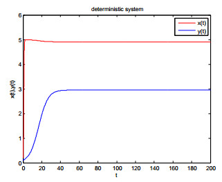
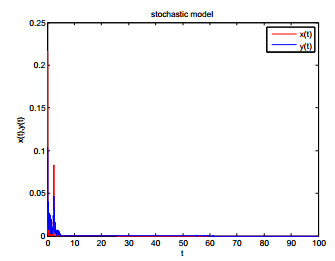
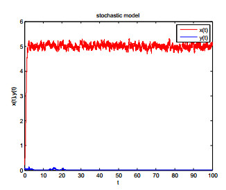
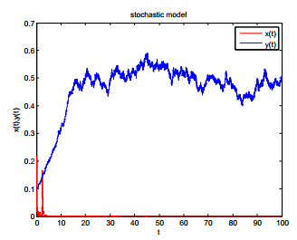
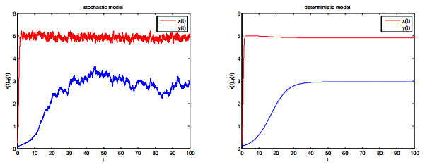
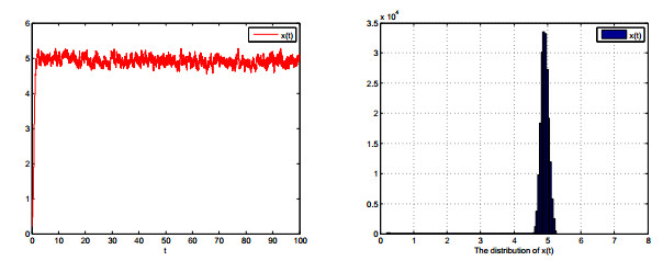
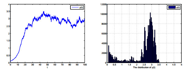
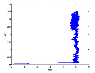
In this paper, a prey-predator model with modified Leslie-Gower and simplified Holling-type Ⅳ functional responses is proposed to study the dynamic behaviors. For the deterministic system, we analyze the permanence of the system and the stability of the positive equilibrium point. For the stochastic system, we not only prove the existence and uniqueness of global positive solution, but also discuss the persistence in mean and extinction of the populations. In addition, we find that stochastic system has an ergodic stationary distribution under some parameter constraints. Finally, our theoretical results are verified by numerical simulations.
- permanence,
- positive equilibrium point,
- persistence in mean,
- extinction,
- ergodic stationary distribution
Citation: Lin Li, Wencai Zhao. Deterministic and stochastic dynamics of a modified Leslie-Gower prey-predator system with simplified Holling-type Ⅳ scheme[J]. Mathematical Biosciences and Engineering, 2021, 18(3): 2813-2831. doi: 10.3934/mbe.2021143

Related Papers:

Abstract

In this paper, a prey-predator model with modified Leslie-Gower and simplified Holling-type Ⅳ functional responses is proposed to study the dynamic behaviors. For the deterministic system, we analyze the permanence of the system and the stability of the positive equilibrium point. For the stochastic system, we not only prove the existence and uniqueness of global positive solution, but also discuss the persistence in mean and extinction of the populations. In addition, we find that stochastic system has an ergodic stationary distribution under some parameter constraints. Finally, our theoretical results are verified by numerical simulations.

References

[1]	S. C. Hoyt, Integrated chemical control of insects and biological control of mites on apple in washington, J. Econ. Entomol., 62 (1969), 74–86. doi: 10.1093/jee/62.1.74
[2]	D. J. Wollkind, J. B. Collings, J. A. Logan, Metastability in a temperature-dependent model system for predator-prey mite outbreak interactions on fruit trees, Bull. Math. Biol., 50 (1988), 379–409. doi: 10.1016/S0092-8240(88)90005-5
[3]	J. B. Collings, The effects of the functional response on the bifurcation behavior of a mite predator-prey interaction model, J. Math. Biol, 36 (1997), 149–168. doi: 10.1007/s002850050095
[4]	R. J. Taylor, Predation, New York: Chapman and Hall, (1984).
[5]	M. W.Sabelis, Predation on Spider Mites, Amsterdam: Elsevier, (1985), 103–129.
[6]	W. Sokol, J. A. Howell, Kinetics of phenol oxidation by washed cells, Biotechnol. Bioeng., 23 (1981), 2039–2049. doi: 10.1002/bit.260230909
[7]	B. Gonzalez-Yanez, E. Gonzalez-Olivares, J. Mena-Lorca, Multistability on a Leslie-Gower type predator-prey model with nonmonotonic functional response, In R. Mondaini and R. Dilao (eds.), BIOMAT 2006 - International Symposium on Mathematical and Computational Biology, World Scienti.c Co. Pte. Ltd. (2007), 359–384.
[8]	Y. Li, D. Xiao, Bifurcations of a predator-prey system of Holling and Leslie types, Chaos Soliton. Fract., 34 (2007), 606–620. doi: 10.1016/j.chaos.2006.03.068
[9]	P. Ye, D. Wu, Impacts of strong Allee effect and hunting cooperation for a Leslie-Gower predator-prey system, Chin. J. Phys., 68 (2020), 49–64. doi: 10.1016/j.cjph.2020.07.021
[10]	Y. Liu, Z. Guo, M. E. Smaily, L. Wang, A Leslie-Gower predator-prey model with a free boundary, Discret. Contin. Dyn. Syst., 12 (2019), 2063–2084.
[11]	M.A. Aziz-Alaoui, M. Daher Okiye, Boundedness and global stability for a predator-prey model with modified Leslie-Gower and Holling-type II schemes, Appl. Math. Lett., 16 (2003), 1069–1075. doi: 10.1016/S0893-9659(03)90096-6
[12]	L. Puchuri Medina, E. Gonzalez-Olivares, A. Rojas-Palma, Multistability in a Leslie-Gower type predation model with rational nonmonotonic functional response and generalist predators, Comp. Math. Methods, 2 (2020).
[13]	J. Liu, W. Zhao, The dynamic analysis of a stochastic prey-predator model with Markovian switching and different functional responses, Math. Model. Appl., 7 (2018), 12–21.
[14]	T. Zhang, N. Gao, J. Wang, Z. Jiang, Dynamic system of microbial culture described by impulsive differential equations, Math. Model. Appl., 8 (2019), 1–13.
[15]	X. Lv, X. Meng, Analysis of dynamic behavior for a nonlinear stochastic non-autonomous SIRS model, Math. Model. Appl., 7 (2018), 16–23.
[16]	P. Aguirre, E. Gonzalez-Olivares, S. Torres, Stochastic predator-prey model with Allee effect on preys, Nonlinear Anal.-Real World Appl., 14 (2013), 768–779. doi: 10.1016/j.nonrwa.2012.07.032
[17]	X. Zhao, Z. Zeng, Stationary distribution of a stochastic predator-prey system with stage structure for prey, Phys. A, (2020), 545.
[18]	Q. Liu, D. Jiang, T. Hayat, A. Alsaedi, Dynamical behavior of stochastic predator-prey models with distributed delay and general functional response, Stoch. Anal. Appl., 38 (2020), 403–426. doi: 10.1080/07362994.2019.1695628
[19]	D. Manna, A. Maiti, G.P. Samanta, Deterministic and stochastic analysis of a predator-prey model with Allee effect and herd behaviour, Simulation., 95 (2019), 339–349. doi: 10.1177/0037549718779445
[20]	Q. Liu, D. Jiang, Influence of the fear factor on the dynamics of a stochastic predator-prey model, Appl. Math. Lett., 112 (2021), 106756. doi: 10.1016/j.aml.2020.106756
[21]	C. Xu, Y. Yu, G. Ren, Dynamic analysis of a stochastic predator-prey model with Crowley-Martin functional response, disease in predator, and saturation incidence, J. Comput. Nonlinear Dyn., 15 (2020).
[22]	V. Lakshmikantham, D. D. Bainov, P. S. Simeonov, Theory of impulsive differential equations, Singapore: World Scientific (1989), 265–273.
[23]	F. Chen, Z. Li, Y. Huang, Note on the permanence of a competitive system with infinite delay and feedback controls, Nonlinear Anal. RWA, 8 (2007), 680–687. doi: 10.1016/j.nonrwa.2006.02.006
[24]	L. Arnold, Stochastic differential equations: Theory and applications, Bull. London Math. Soc., 8 (1976), 409.
[25]	P. S. Mandal, M. Banerjee, Stochastic persistence and stationary distribution in a Holling-Tanner type prey-predator model, Phys. A, 391 (2012), 1216–1233. doi: 10.1016/j.physa.2011.10.019
[26]	C. Ji, D. Jiang, N. Shi, Analysis of a predator-prey model with modified Leslie-Gower and Holling-type II schemes with stochastic perturbation, J. Math. Anal. Appl., 359 (2009), 482–498. doi: 10.1016/j.jmaa.2009.05.039
[27]	D. Zhou, M. Liu, Z. Liu, Persistence and extinction of a stochastic predator-prey model with modified Leslie-Gower and Holling-type II schemes, Adv. Differ. Equ., 2020 (2020).
[28]	D. Xu, M. Liu, X. Xu, Analysis of a stochastic predator-prey system with modified Leslie-Gower and Holling-type IV schemes, Phys. A, 537 (2019), 122761.
[29]	H. Li, F. Cong, Dynamics of a stochastic Holling-Tanner predator-prey model, Phys. A, 531 (2019), 121761. doi: 10.1016/j.physa.2019.121761

Reader Comments

Your name:*

Email:*
© 2021 the Author(s), licensee AIMS Press. This is an open access article distributed under the terms of the Creative Commons Attribution License (http://creativecommons.org/licenses/by/4.0)