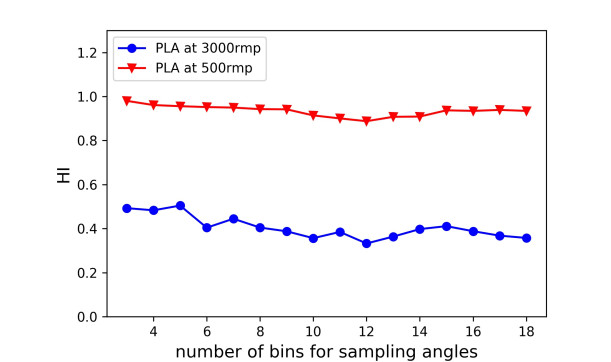
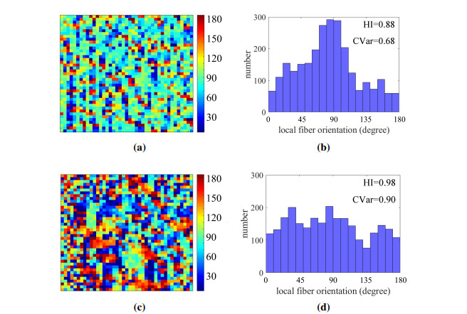
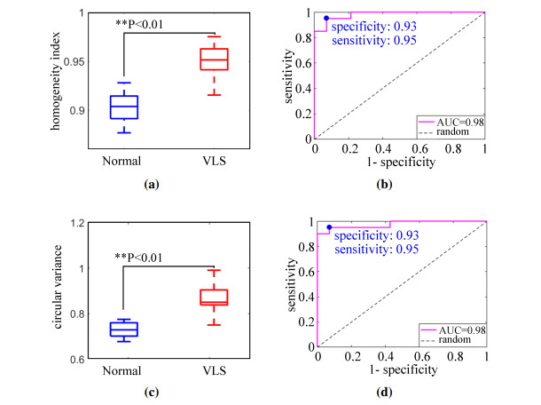
Collagen alignment has shown clinical significance in a variety of diseases. For instance, vulvar lichen sclerosus (VLS) is characterized by homogenization of collagen fibers with increasing risk of malignant transformation. To date, a variety of imaging techniques have been developed to visualize collagen fibers. However, few works focused on quantifying the alignment quality of collagen fiber. To assess the level of disorder of local fiber orientation, the homogeneity index (HI) based on limiting entropy is proposed as an indicator of disorder. Our proposed methods are validated by verification experiments on Poly Lactic Acid (PLA) filament phantoms with controlled alignment quality of fibers. A case study on 20 VLS tissue biopsies and 14 normal tissue biopsies shows that HI can effectively characterize VLS tissue from normal tissue (P < 0.01). The classification results are very promising with a sensitivity of 93% and a specificity of 95%, which indicated that our method can provide quantitative assessment for the alignment quality of collagen fibers in VLS tissue and aid in improving histopathological examination of VLS.
Citation: Yingjie Qu, Zachary J. Smith, Kelly Tyler, Shufang Chang, Shuwei Shen, Mingzhai Sun, Ronald X. Xu. Applying limiting entropy to quantify the alignment of collagen fibers by polarized light imaging[J]. Mathematical Biosciences and Engineering, 2021, 18(3): 2331-2356. doi: 10.3934/mbe.2021118
Collagen alignment has shown clinical significance in a variety of diseases. For instance, vulvar lichen sclerosus (VLS) is characterized by homogenization of collagen fibers with increasing risk of malignant transformation. To date, a variety of imaging techniques have been developed to visualize collagen fibers. However, few works focused on quantifying the alignment quality of collagen fiber. To assess the level of disorder of local fiber orientation, the homogeneity index (HI) based on limiting entropy is proposed as an indicator of disorder. Our proposed methods are validated by verification experiments on Poly Lactic Acid (PLA) filament phantoms with controlled alignment quality of fibers. A case study on 20 VLS tissue biopsies and 14 normal tissue biopsies shows that HI can effectively characterize VLS tissue from normal tissue (P < 0.01). The classification results are very promising with a sensitivity of 93% and a specificity of 95%, which indicated that our method can provide quantitative assessment for the alignment quality of collagen fibers in VLS tissue and aid in improving histopathological examination of VLS.

| [1] |
G. Ramachandran, Molecular structure of collagen, Int. Rev. Connect Tissue Res., 1 (1963), 127-182. doi: 10.1016/B978-1-4831-6755-8.50009-7

|
| [2] |
M. D. Shoulders, R. T. Raines, Collagen structure and stability, Annu. Rev. Biochem., 78 (2009), 929-958. doi: 10.1146/annurev.biochem.77.032207.120833
|
| [3] | P. Berillis, The role of collagen in the aorta's structure, Open Circ. Vasc. J., 6. |
| [4] | C. Stecco, W. Hammer, A. Vleeming, R. De Caro, Functional Atlas of the Human Fascial System, Churchill Livingstone, 2015. |
| [5] | K. Gelse, E. Pöschl, T. Aigner, Collagens—structure, function, and biosynthesis, Adv. Drug Deliver Rev., 55 (2003), 1531-1546. |
| [6] |
A. Pierangelo, A. Nazac, A. Benali, P. Validire, H. Cohen, T. Novikova, et al., Polarimetric imaging of uterine cervix: a case study, Opt. Express, 21 (2013), 14120-14130. doi: 10.1364/OE.21.014120
|
| [7] |
A. E. Woessner, J. D. McGee, J. D. Jones, K. P. Quinn, Characterizing differences in the collagen fiber organization of skin wounds using quantitative polarized light imaging, Wound Repair Regen., 27 (2019), 711-714. doi: 10.1111/wrr.12758
|
| [8] |
J. K. Pijanka, B. Coudrillier, K. Ziegler, T. Sorensen, K. M. Meek, T. D. Nguyen, et al., Quantitative mapping of collagen fiber orientation in non-glaucoma and glaucoma posterior human sclerae, Invest. Ophth. Vis. Sci., 53 (2012), 5258-5270. doi: 10.1167/iovs.12-9705
|
| [9] |
H. de Vries, D. Enomoto, J. van Marle, P. van Zuijlen, J. Mekkes, J. Bos, Dermal organization in scleroderma: the fast fourier transform and the laser scatter method objectify fibrosis in nonlesional as well as lesional skin, Lab. Invest., 80 (2000), 1281-1289, doi: 10.1038/labinvest.3780136
|
| [10] |
M. Conklin, J. Eickhoff, K. Riching, C. Pehlke, K. Eliceiri, P. Provenzano, et al., Aligned collagen is a prognostic signature for survival in human breast carcinoma, AM. J. Pathol., 178 (2011), 1221-1232. doi: 10.1016/j.ajpath.2010.11.076
|
| [11] | O. Nadiarnykh, R. B. Lacomb, M. A. Brewer, P. J. Campagnola, Alterations of the extracellular matrix in ovarian cancer studied by second harmonic generation imaging microscopy, BMC. Cancer, 10 (2009), 94-94. |
| [12] | J. Powell, F. Wojnarowska, Lichen sclerosus, Lancet, 353 (1999), 1777-1783. |
| [13] | G. L. Tasker, F. Wojnarowska, Lichen sclerosus, Clin. Exp. Dermatol., 28 (2003), 128-133. |
| [14] |
D. Suurmond, Lichen sclerosus et atrophicus of the vulva, JAMA. Dermatol., 90 (1964), 143-152. doi: 10.1001/archderm.1964.01600020011002
|
| [15] |
E. G. Wallace, R. Nomland, Lichen sclerosus et atrophicus of the vulva, Arch. Derm. Syphilol., 57 (1948), 240-254. doi: 10.1001/archderm.1948.01520140102013
|
| [16] | J. Powell, F. Wojnarowska, Lichen sclerosus, Lancet, 353 (1999), 1777-1783. |
| [17] |
M. C. Bleeker, P. J. Visser, L. I. Overbeek, M. van Beurden, J. Berkhof, Lichen sclerosus: Incidence and risk of vulvar squamous cell carcinoma, Cancer Epidemiol. Biomarkers Prev., 25 (2016), 1224-1230. doi: 10.1158/1055-9965.EPI-16-0019
|
| [18] |
E. G. Friedrich, N. K. MacLaren, Genetic aspects of vulvar lichen sclerosus, AM. J. Obstet. Gynecol., 150 (1984), 161-166. doi: 10.1016/S0002-9378(84)80008-3
|
| [19] |
L. Niamh, S. Naveen, B. Hazel, Diagnosis of vulval inflammatory dermatoses: A pathological study with clinical correlation, INT. J. Gynecol. Pathol., 28 (2009), 554-558. doi: 10.1097/PGP.0b013e3181a9fb0d
|
| [20] |
L. Sclerosus, Vulvar nonneoplastic epithelial disorders, INT. J. Gynecol. Obstet., 60 (1998), 181-188. doi: 10.1016/S0020-7292(97)90227-7
|
| [21] |
H. K. Haefner, N. Z. Aldrich, V. K. Dalton, H. M. Gagné, S. B. Marcus, D. A. Patel, et al., The impact of vulvar lichen sclerosus on sexual dysfunction, J. Womens Health, 23 (2014), 765-770. doi: 10.1089/jwh.2014.4805
|
| [22] |
J. M. Krapf, L. Mitchell, M. A. Holton, A. T. Goldstein, Vulvar lichen sclerosus: Current perspectives, IN. J. Womens Health, 12 (2020), 11. doi: 10.2147/IJWH.S191200
|
| [23] | C. Lansdorp, K. van~den Hondel, I. Korfage, M. van Gestel, W. van der Meijden, Quality of life in dutch women with lichen sclerosus, Brit. J. Dermatol., 168 (2013), 787-793. |
| [24] | M. Pešek, J. Bouda, non-neoplastic epithelial disorders of the vulva - lichen sclerosus, Ceska. Gynekol., 79 (2014), 57-63. |
| [25] | L. S. Jensen, A. Bygum, Childhood lichen sclerosus is a rare but important diagnosis, Dan. Med. J., 59 (2012), A4424. |
| [26] | S. Cooper, X. -H. Gao, J. Powell, F. Wojnarowska, Does treatment of vulvar lichen sclerosus influence its prognosis?, JAMA. Dermatol., 140 (2004), 702-706. |
| [27] |
S. K. Fistarol, P. H. Itin, Diagnosis and treatment of lichen sclerosus, Am. J. Clin. Dermatol., 14 (2013), 27-47. doi: 10.1007/s40257-012-0006-4
|
| [28] | J. Hewitt, Histologic criteria for lichen sclerosus of the vulva, J. Reprod. Med., 31 (1986), 781-787. |
| [29] | J. A. Carlson, P. Lamb, J. Malfetano, R. A. Ambros, J. M. Mihm, Clinicopathologic comparison of vulvar and extragenital lichen sclerosus: histologic variants, evolving lesions, and etiology of 141 cases, Mod. Pathol., 11 (1998), 844-854. |
| [30] |
H. L. d. Almeida, E. d. B. C. Bicca, J. d. A. Breunig, N. M. Rocha, R. M. E. Silva, Scanning electron microscopy of lichen sclerosus, An. Bras. Dermatol., 88 (2013), 247-249. doi: 10.1590/S0365-05962013000200011
|
| [31] |
A. Keikhosravi, Y. Liu, C. Drifka, K. M. Woo, A. Verma, R. Oldenbourg, et al., Quantification of collagen organization in histopathology samples using liquid crystal based polarization microscopy, Biomed. Opt. Express, 8 (2017), 4243-4256. doi: 10.1364/BOE.8.004243
|
| [32] |
S. Bancelin, A. Nazac, B. H. Ibrahim, P. Dokládal, E. Decencière, B. Teig, et al., Determination of collagen fiber orientation in histological slides using mueller microscopy and validation by second harmonic generation imaging, Opt. Express, 22 (2014), 22561-22574. doi: 10.1364/OE.22.022561
|
| [33] |
M. Sivaguru, S. Durgam, R. Ambekar, D. Luedtke, G. Fried, A. Stewart, et al., Quantitative analysis of collagen fiber organization in injured tendons using fourier transform-second harmonic generation imaging, Opt. Express, 18 (2010), 24983-24993. doi: 10.1364/OE.18.024983
|
| [34] |
X. Chen, O. Nadiarynkh, S. Plotnikov, P. J. Campagnola, Second harmonic generation microscopy for quantitative analysis of collagen fibrillar structure, Nat. Protoc., 7 (2012), 654. doi: 10.1038/nprot.2012.009
|
| [35] |
S. Jiao, L. V. Wang, Two-dimensional depth-resolved mueller matrix of biological tissue measured with double-beam polarization-sensitive optical coherence tomography, Opt. Lett., 27 (2002), 101-103. doi: 10.1364/OL.27.000101
|
| [36] |
A. J. Schriefl, A. J. Reinisch, S. Sankaran, D. M. Pierce, G. A. Holzapfel, Quantitative assessment of collagen fibre orientations from two-dimensional images of soft biological tissues, J. R. Soc. Interface, 9 (2012), 3081-3093. doi: 10.1098/rsif.2012.0339
|
| [37] |
T. Starborg, N. S. Kalson, Y. Lu, A. Mironov, T. F. Cootes, D. F. Holmes, et al., Using transmission electron microscopy and 3view to determine collagen fibril size and three-dimensional organization, Nat. Protoc., 8 (2013), 1433-48. doi: 10.1038/nprot.2013.086
|
| [38] |
M. S. Sacks, D. B. Smith, E. D. Hiester, A small angle light scattering device for planar connective tissue microstructural analysis, Ann. Biomed. Eng., 25 (1997), 678-89. doi: 10.1007/BF02684845
|
| [39] |
E. Brown, T. McKee, E. diTomaso, A. Pluen, B. Seed, Y. Boucher, et al., Dynamic imaging of collagen and its modulation in tumors in vivo using second-harmonic generation, Nat. Med., 9 (2003), 796-800. doi: 10.1038/nm879
|
| [40] |
P. Campagnola, C. -Y. Dong, Second harmonic generation microscopy: principles and applications to disease diagnosis, Laser Photon Rev., 5 (2011), 13-26. doi: 10.1002/lpor.200910024
|
| [41] |
S. L. Jacques, J. C. Ramella-Roman, K. Lee, Imaging skin pathology with polarized light, J. Biomed. Opt., 7 (2002), 329-341. doi: 10.1117/1.1484498
|
| [42] |
S. L. Jacques, S. Roussel, R. V. Samatham, Polarized light imaging specifies the anisotropy of light scattering in the superficial layer of a tissue, J. Biomed. Opt., 21 (2016), 071115. doi: 10.1117/1.JBO.21.7.071115
|
| [43] |
X. Li, J. C. Ranasinghesagara, G. Yao, Polarization-sensitive reflectance imaging in skeletal muscle, Opt. Express, 16 (2008), 9927-9935. doi: 10.1364/OE.16.009927
|
| [44] |
B. Yang, J. Lesicko, M. Sharma, M. Hill, M. S. Sacks, J. W. Tunnell, Polarized light spatial frequency domain imaging for non-destructive quantification of soft tissue fibrous structures, Biomed. Opt. Express, 6 (2015), 1520-1533. doi: 10.1364/BOE.6.001520
|
| [45] |
R. Liao, N. Zeng, X. Jiang, D. Li, T. Yun, Y. He, et al., Rotating linear polarization imaging technique for anisotropic tissues, J. Biomed. Opt., 15 (2010), 036014. doi: 10.1117/1.3442730
|
| [46] |
P. J. Wu, J. T. Walsh, Stokes polarimetry imaging of rat tail tissue in a turbid medium: degree of linear polarization image maps using incident linearly polarized light, J. Biomed. Opt., 11 (2006), 014031. doi: 10.1117/1.2162851
|
| [47] | K. P. Balanda, H. L. MacGillivray, Kurtosis: A critical review, Am. Stat., 42 (1988), 111-119. |
| [48] |
J. Jensen, I. Currie, New method for estimating the dykstra-parsons coefficient to characterize reservoir heterogeneity, SPE. Reserv. Eng., 5 (1990), 369-374. doi: 10.2118/17364-PA
|
| [49] | S. R. Jammalamadaka, A. Sengupta, Topics in circular statistics, vol. 5, world scientific, 2001. |
| [50] |
C. E. Shannon, A mathematical theory of communication, Bell Syst. Tech. J., 27 (1948), 379-423. doi: 10.1002/j.1538-7305.1948.tb01338.x
|
| [51] | R. B. Ash, Information Theory, Dover Publications Inc., New York, 1990. |
| [52] | McGraw-Hill, McGraw-Hill Concise Encyclopedia of Chemistry, McGraw-Hill Professional Pub, 2004. |
| [53] | G. Ducourthial, J. -s. Affagard, M. Schmeltz, X. Solinas, M. Lopez-Poncelas, C. Bonod-Bidaud, et al., Monitoring dynamic collagen reorganization during skin stretching with fast polarization-resolved second harmonic generation imaging, J. Biophoton., 12 (2019), e201800336. |
| [54] |
J. P. Chiverton, O. Ige, S. J. Barnett, T. Parry, Multiscale shannon's entropy modeling of orientation and distance in steel fiber micro-tomography data, IEEE. Trans. Image Process, 26 (2017), 5284-5297. doi: 10.1109/TIP.2017.2722234
|
| [55] | E. T. Jaynes, Information theory and statistical mechanics, Probability Theory: The Logic of Science, Cambridge University Press, 2003 |
| [56] | M. Born, E. Wolf, Principles of optics: electromagnetic theory of propagation, interference and diffraction of light, Elsevier, 2013. |
| [57] |
S. Shen, H. Wang, Y. Qu, K. Huang, G. Liu, Z. Chen, et al., Simulating orientation and polarization characteristics of dense fibrous tissue by electrostatic spinning of polymeric fibers, Biomed. Opt. Express, 10 (2019), 571-583. doi: 10.1364/BOE.10.000571
|
| [58] |
Y. Chen, J. Lin, Y. Fei, H. Wang, W. Gao, Preparation and characterization of electrospinning pla/curcumin composite membranes, Fiber Polym., 11 (2010), 1128-1131. doi: 10.1007/s12221-010-1128-z
|
| [59] |
P. Katta, M. Alessandro, R. Ramsier, G. Chase, Continuous electrospinning of aligned polymer nanofibers onto a wire drum collector, Nano Lett., 4 (2004), 2215-2218. doi: 10.1021/nl0486158
|
| [60] |
X. Zong, K. Kim, D. Fang, S. Ran, B. S. Hsiao, B. Chu, Structure and process relationship of electrospun bioabsorbable nanofiber membranes, Polymer, 43 (2002), 4403-4412. doi: 10.1016/S0032-3861(02)00275-6
|
| [61] |
M. M. Arras, C. Grasl, H. Bergmeister, H. Schima, Electrospinning of aligned fibers with adjustable orientation using auxiliary electrodes, Sci. Technol. Adv. Mat., 13 (2012), 035008. doi: 10.1088/1468-6996/13/3/035008
|
| [62] |
M. V. Kakade, S. Givens, K. Gardner, K. H. Lee, D. B. Chase, J. F. Rabolt, Electric field induced orientation of polymer chains in macroscopically aligned electrospun polymer nanofibers, J. Am. Chem. Soc., 129 (2007), 2777-2782. doi: 10.1021/ja065043f
|
| [63] |
G. Mathew, J. Hong, J. Rhee, D. Leo, C. Nah, Preparation and anisotropic mechanical behavior of highly-oriented electrospun poly (butylene terephthalate) fibers, J. Appl. Polym. Sci., 101 (2006), 2017-2021. doi: 10.1002/app.23762
|
| [64] | M. Wood, N. Vurgun, M. Wallenburg, I. Vitkin, Effects of formalin fixation on tissue optical polarization properties, Phys. Med. Biol., 56 (2011), N115. |
| [65] |
N. -J. Jan, J. L. Grimm, H. Tran, K. L. Lathrop, G. Wollstein, R. A. Bilonick, et al., Polarization microscopy for characterizing fiber orientation of ocular tissues, Biomed. Opt. Express, 6 (2015), 4705-4718. doi: 10.1364/BOE.6.004705
|
| [66] |
J. Frost, L. Ludeman, K. Hillaby, R. Gornall, G. Lloyd, C. Kendall, et al., Raman spectroscopy and multivariate analysis for the non invasive diagnosis of clinically inconclusive vulval lichen sclerosus, Analyst, 142 (2017), 1200-1206. doi: 10.1039/C6AN02009G
|
Figures(11) / Tables(1)

Yingjie Qu, Zachary J. Smith, Kelly Tyler, Shufang Chang, Shuwei Shen, Mingzhai Sun, Ronald X. Xu. Applying limiting entropy to quantify the alignment of collagen fibers by polarized light imaging[J]. Mathematical Biosciences and Engineering, 2021, 18(3): 2331-2356. doi: 10.3934/mbe.2021118


 DownLoad: