Retinal blood vessel segmentation from fundus image using an efficient multiscale directional representation technique Bendlets

Rafsanjany Kushol; Md. Hasanul Kabir; M. Abdullah-Al-Wadud; Md Saiful Islam; Rafsanjany Kushol; Md. Hasanul Kabir; M. Abdullah-Al-Wadud; Md Saiful Islam

doi:10.3934/mbe.2020394

Mathematical Biosciences and Engineering

2020, Volume 17, Issue 6: 7751-7771. doi: 10.3934/mbe.2020394

Previous Article Next Article

Research article Special Issues

Retinal blood vessel segmentation from fundus image using an efficient multiscale directional representation technique Bendlets

1.
Department of Computing Science, University of Alberta, Edmonton, AB, Canada
2.
Department of Computer Science and Engineering, Islamic University of Technology, Dhaka, Bangladesh
3.
Department of Software Engineering, King Saud University, Riyadh, Saudi Arabia
4.
Department of Computer Science, King Saud University, Riyadh, Saudi Arabia

Received: 27 July 2020 Accepted: 12 October 2020 Published: 06 November 2020

The improper circulation of blood flow inside the retinal vessel is the primary source of most of the optical disorders including partial vision loss and blindness. Accurate blood vessel segmentation of the retinal image is utilized for biometric identification, computer-assisted laser surgical procedure, automatic screening, and diagnosis of ophthalmologic diseases like Diabetic retinopathy, Age-related macular degeneration, Hypertensive retinopathy, and so on. Proper identification of retinal blood vessels at its early stage assists medical experts to take expedient treatment procedures which could mitigate potential vision loss. This paper presents an efficient retinal blood vessel segmentation approach where a 4-D feature vector is constructed by the outcome of Bendlet transform, which can capture directional information much more efficiently than the traditional wavelets. Afterward, a bunch of ensemble classifiers is applied to find out the best possible result of whether a pixel falls inside a vessel or non-vessel segment. The detailed and comprehensive experiments operated on two benchmark and publicly available retinal color image databases (DRIVE and STARE) prove the effectiveness of the proposed approach where the average accuracy for vessel segmentation accomplished approximately 95%. Furthermore, in comparison with other promising works on the aforementioned databases demonstrates the enhanced performance and robustness of the proposed method.
- Bendlets,
- retinal blood vessel,
- ensemble classifier,
- medical image segmentation,
- contrast enhancement,
- multi-resolution,
- multi-scale transform
Citation: Rafsanjany Kushol, Md. Hasanul Kabir, M. Abdullah-Al-Wadud, Md Saiful Islam. Retinal blood vessel segmentation from fundus image using an efficient multiscale directional representation technique Bendlets[J]. Mathematical Biosciences and Engineering, 2020, 17(6): 7751-7771. doi: 10.3934/mbe.2020394

Related Papers:

Abstract

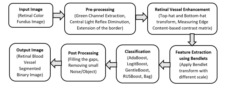
The improper circulation of blood flow inside the retinal vessel is the primary source of most of the optical disorders including partial vision loss and blindness. Accurate blood vessel segmentation of the retinal image is utilized for biometric identification, computer-assisted laser surgical procedure, automatic screening, and diagnosis of ophthalmologic diseases like Diabetic retinopathy, Age-related macular degeneration, Hypertensive retinopathy, and so on. Proper identification of retinal blood vessels at its early stage assists medical experts to take expedient treatment procedures which could mitigate potential vision loss. This paper presents an efficient retinal blood vessel segmentation approach where a 4-D feature vector is constructed by the outcome of Bendlet transform, which can capture directional information much more efficiently than the traditional wavelets. Afterward, a bunch of ensemble classifiers is applied to find out the best possible result of whether a pixel falls inside a vessel or non-vessel segment. The detailed and comprehensive experiments operated on two benchmark and publicly available retinal color image databases (DRIVE and STARE) prove the effectiveness of the proposed approach where the average accuracy for vessel segmentation accomplished approximately 95%. Furthermore, in comparison with other promising works on the aforementioned databases demonstrates the enhanced performance and robustness of the proposed method.

References

[1]	A. M. Joussen, T. W. Gardner, B. Kirchhof, S. J. Ryan, Retinal vascular disease, Springer, 2007.
[2]	S. Chaudhuri, S. Chatterjee, N. Katz, M. Nelson, M. Goldbaum, Detection of blood vessels in retinal images using two-dimensional matched filters, IEEE Trans. Med. Imaging, 8 (1989), 263-269. doi: 10.1109/42.34715
[3]	M. E. Martínez-Pérez, A. D. Hughes, A. V. Stanton, S. A. Thom, A. A. Bharath, K. H. Parker, Retinal blood vessel segmentation by means of scale-space analysis and region growing, in Inter-national Conference on Medical Image Computing and Computer-Assisted Intervention, Springer, (1999), 90-97.
[4]	A. M. Mendonca, A. Campilho, Segmentation of retinal blood vessels by combining the detection of centerlines and morphological reconstruction, IEEE Trans. Med. Imaging, 25 (2006), 1200-1213. doi: 10.1109/TMI.2006.879955
[5]	N. Brancati, M. Frucci, D. Gragnaniello, D. Riccio, Retinal vessels segmentation based on a con-volutional neural network, in Iberoamerican Congress on Pattern Recognition, Springer, (2017), 119-126.
[6]	E. J. Candes, D. L. Donoho, Curvelets: A surprisingly effective nonadaptive representationfor objects with edges, Technical report, Stanford Uni Ca Dept of Statistics, 2000.
[7]	M. N. Do, M. Vetterli, The contourlet transform: an efficient directional multiresolution image representation, IEEE Trans. Image Proc., 14 (2005), 2091-2106. doi: 10.1109/TIP.2005.859376
[8]	W.-Q. Lim, The discrete shearlet transform: a new directional transform and compactly supported shearlet frames., IEEE Trans. Image Proc., 19 (2010), 1166-1180. doi: 10.1109/TIP.2010.2041410
[9]	C. Lessig, P. Petersen, M. Schäfer, Bendlets: A second-order shearlet transform with bent elements, Appl. Comput. Harmonic Anal., 46 (2019), 384-399. doi: 10.1016/j.acha.2017.06.002
[10]	A. Hoover, V. Kouznetsova, M. Goldbaum, Locating blood vessels in retinal images by piecewise threshold probing of a matched filter response, IEEE Trans. Med. Imaging, 19 (2000), 203-210. doi: 10.1109/42.845178
[11]	B. Zhang, L. Zhang, L. Zhang, F. Karray, Retinal vessel extraction by matched filter with first-order derivative of gaussian, Comput. Biol. Med., 40 (2010), 438-445. doi: 10.1016/j.compbiomed.2010.02.008
[12]	J. Odstrcilik, R. Kolar, A. Budai, J. Hornegger, J. Jan, J. Gazarek, et al., Retinal vessel segmentation by improved matched filtering: evaluation on a new high-resolution fundus image database, IET Image Proc., 7 (2013), 373-383.
[13]	T. Chakraborti, D. K. Jha, A. S. Chowdhury, X. Jiang, A self-adaptive matched filter for retinal blood vessel detection, Mach. Vision Appl., 26 (2015), 55-68. doi: 10.1007/s00138-014-0636-z
[14]	M. Vlachos, E. Dermatas, Multi-scale retinal vessel segmentation using line tracking, Comput. Med Imaging Graphics, 34 (2010), 213-227. doi: 10.1016/j.compmedimag.2009.09.006
[15]	U. T. Nguyen, A. Bhuiyan, L. A. Park, K. Ramamohanarao, An effective retinal blood vessel segmentation method using multi-scale line detection, Pattern Recognit., 46 (2013), 703-715. doi: 10.1016/j.patcog.2012.08.009
[16]	Y. Hou, Automatic segmentation of retinal blood vessels based on improved multiscale line detection, J. Comput. Sci. Eng.ng, 8 (2014), 119-128. doi: 10.5626/JCSE.2014.8.2.119
[17]	K. Yue, B. Zou, Z. Chen, Q. Liu, Improved multi-scale line detection method for retinal blood vessel segmentation, IET Image Proc., 12 (2018), 1450-1457. doi: 10.1049/iet-ipr.2017.1071
[18]	M. S. Miri, A. Mahloojifar, Retinal image analysis using curvelet transform and multistructure elements morphology by reconstruction, IEEE Trans. Biomed. Eng., 58 (2011), 1183-1192. doi: 10.1109/TBME.2010.2097599
[19]	M. M. Fraz, S. A. Barman, P. Remagnino, A. Hoppe, A. Basit, B. Uyyanonvara, et al., An approach to localize the retinal blood vessels using bit planes and centerline detection, Comput. Methods Programs Biomed., 108 (2012), 600-616.
[20]	E. Imani, M. Javidi, H. R. Pourreza, Improvement of retinal blood vessel detection using morphological component analysis, Comput. Methods Programs Biomed., 118 (2015), 263-279. doi: 10.1016/j.cmpb.2015.01.004
[21]	J. Gao, G. Chen, W. Lin, An effective retinal blood vessel segmentation by using automatic random walks based on centerline extraction, BioMed Res. Int., 2020 (2020).
[22]	E. Ricci, R. Perfetti, Retinal blood vessel segmentation using line operators and support vector classification, IEEE Trans. Med. Imaging, 26 (2007), 1357-1365. doi: 10.1109/TMI.2007.898551
[23]	D. Marín, A. Aquino, M. E. Gegúndez-Arias, J. M. Bravo, A new supervised method for blood vessel segmentation in retinal images by using gray-level and moment invariants-based features, IEEE Trans. Med. Imaging, 30 (2011), 146-158. doi: 10.1109/TMI.2010.2064333
[24]	Z. Fan, Y. Rong, J. Lu, J. Mo, F. Li, X. Cai, et al., Automated blood vessel segmentation in fundus image based on integral channel features and random forests, 2016 12th World Congress on Intelligent Control and Automation (WCICA), IEEE, 2016.
[25]	J. V. Soares, J. J. Leandro, R. M. Cesar, H. F. Jelinek, M. J. Cree, Retinal vessel segmentation using the 2-d gabor wavelet and supervised classification, IEEE Trans. Med. Imaging, 25 (2006), 1214-1222. doi: 10.1109/TMI.2006.879967
[26]	L. Xu, S. Luo, A novel method for blood vessel detection from retinal images, Biomed. Eng. online, 9 (2010), 1.
[27]	M. M. Fraz, P. Remagnino, A. Hoppe, B. Uyyanonvara, A. R. Rudnicka, C. G. Owen, et al., An ensemble classification-based approach applied to retinal blood vessel segmentation, IEEE Trans. Biomed. Eng., 59 (2012), 2538-2548.
[28]	F. Ghadiri, S. M. Zabihi, H. R. Pourreza, T. Banaee, A novel method for vessel detection using contourlet transform, 2012 National Conference on Communications (NCC), IEEE, 2012.
[29]	P. Bankhead, C. N. Scholfield, J. G. McGeown, T. M. Curtis, Fast retinal vessel detection and measurement using wavelets and edge location refinement, PloS one, 7 (2012), e32435.
[30]	G. Azzopardi, N. Strisciuglio, M. Vento, N. Petkov, Trainable cosfire filters for vessel delineation with application to retinal images, Med. Image Anal., 19 (2015), 46-57. doi: 10.1016/j.media.2014.08.002
[31]	F. Levet, M. A. Duval-Poo, E. De Vito, F. Odone, Retinal image analysis with shearlets, in STAG, (2016), 151-156.
[32]	B. Khomri, A. Christodoulidis, L. Djerou, M. C. Babahenini, F. Cheriet, Retinal blood vessel segmentation using the elite-guided multi-objective artificial bee colony algorithm, IET Image Proc., 12 (2018), 2163-2171. doi: 10.1049/iet-ipr.2018.5425
[33]	M. Z. Alom, M. Hasan, C. Yakopcic, T. M. Taha, V. K. Asari, Recurrent residual convolutional neural network based on u-net (r2u-net) for medical image segmentation, Forthcoming, 2018.
[34]	S. Y. Shin, S. Lee, I. D. Yun, K. M. Lee, Deep vessel segmentation by learning graphical connectivity, Med. Image Anal., 58 (2019), 101556.
[35]	M. Al-Rawi, M. Qutaishat, M. Arrar, An improved matched filter for blood vessel detection of digital retinal images, Comput. Biol. Med., 37 (2007), 262-267. doi: 10.1016/j.compbiomed.2006.03.003
[36]	L. Li, M. Verma, Y. Nakashima, H. Nagahara, R. Kawasaki, Iternet: Retinal image segmentation utilizing structural redundancy in vessel networks, in The IEEE Winter Conference on Applications of Computer Vision, (2020), 3656-3665.
[37]	R. Kushol, M. H. Kabir, M. S. Salekin, A. A. Rahman, Contrast enhancement by top-hat and bottom-hat transform with optimal structuring element: Application to retinal vessel segmentation, in International Conference Image Analysis and Recognition, Springer, (2017), 533-540.
[38]	R. Kushol, M. N. Raihan, M. S. Salekin, A. A. Rahman, Contrast enhancement of medical x-ray image using morphological operators with optimal structuring element, Forthcoming, 2019.
[39]	M. Niemeijer, J. Staal, B. van Ginneken, M. Loog, M. D. Abramoff, Comparative study of retinal vessel segmentation methods on a new publicly available database, Proceedings of SPIE. Belling-ham: Society of Photo-Optical Instrumentation Engineers Press, 2004.
[40]	V. M. Saffarzadeh, A. Osareh, B. Shadgar, Vessel segmentation in retinal images using multi-scale line operator and k-means clustering, J. Med. Signals Sens., 4 (2014), 122.

Reader Comments

Your name:*

Email:*
© 2020 the Author(s), licensee AIMS Press. This is an open access article distributed under the terms of the Creative Commons Attribution License (http://creativecommons.org/licenses/by/4.0)