Vaccination strategy is considered as the most cost-effective intervention measure for controlling diseases. It will strengthen the immunity and reduce the risks of infections. In this paper, a new delayed epidemic model with interim-immune and mixed vaccination strategy is studied. The diseasefree periodic solution is obtained by twice stroboscopic mapping and the corresponding dynamical behavior is analyzed. We determine a threshold parameter R1, the disease-free periodic solution is proved to be global attractive if R1 < 1. We also establish a threshold parameter R2 for the permanence of the model, i.e., if R2 > 1, the infectious disease will exist persistently. Then, we provide numerical simulations to illustrate our theoretical results intuitively. In particular, a practical application for newtype TB vaccine under mixed vaccination strategy is presented, based on the proposed theory and the data reported by NBSC. The mixed vaccination strategy can achieve the End TB goal formulated by WHO in limited time. Our study will help public health agency to design mixed control strategy which can reduce the burden of infectious diseases.
Citation: Siyu Liu, Mingwang Shen, Yingjie Bi. Global asymptotic behavior for mixed vaccination strategy in a delayed epidemic model with interim-immune[J]. Mathematical Biosciences and Engineering, 2020, 17(4): 3601-3617. doi: 10.3934/mbe.2020203
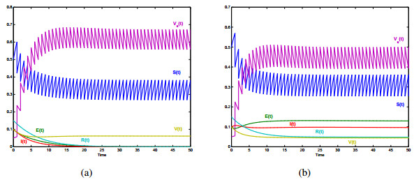
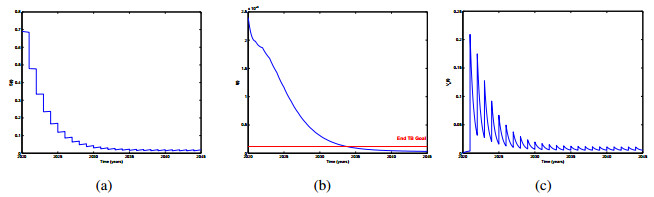
Vaccination strategy is considered as the most cost-effective intervention measure for controlling diseases. It will strengthen the immunity and reduce the risks of infections. In this paper, a new delayed epidemic model with interim-immune and mixed vaccination strategy is studied. The diseasefree periodic solution is obtained by twice stroboscopic mapping and the corresponding dynamical behavior is analyzed. We determine a threshold parameter R1, the disease-free periodic solution is proved to be global attractive if R1 < 1. We also establish a threshold parameter R2 for the permanence of the model, i.e., if R2 > 1, the infectious disease will exist persistently. Then, we provide numerical simulations to illustrate our theoretical results intuitively. In particular, a practical application for newtype TB vaccine under mixed vaccination strategy is presented, based on the proposed theory and the data reported by NBSC. The mixed vaccination strategy can achieve the End TB goal formulated by WHO in limited time. Our study will help public health agency to design mixed control strategy which can reduce the burden of infectious diseases.

| [1] | World Health Organization, The world health report 2007-A safer future: global public health securit in the 21st century, Geneva, 2007. |
| [2] |
A. Henao-Restrepo, I. Longini, M. Egger, N. Dean, W. Edmunds, A. Camacho, et al., Efficacy and effectiveness of an rVSV-vectored vaccine expressing Ebola surface glycoprotein: interim results form the Guinea ring vaccination cluster-randomised trial, Lancet, 386 (2015), 857-866. doi: 10.1016/S0140-6736(15)61117-5

|
| [3] | I. Al-Darabsah, Y. Yuan, A time-delayed epidemic model for Ebola disease transmission, Appl. Math. Comput., 290 (2016), 307-325. |
| [4] | M. De la Sen, A. Ibeas, S. Alonso-Quesada, R. Nistal, On a new epidemic model with asymptomatic and dead-infective subpopulations with feedback controls useful for Ebola disease, Discrete Dyn. Nat. Soc., 2017 (2017), 1-22. |
| [5] | World Health Organization, WHO adapts Ebola vaccination strategy in the Democratic Republic of the Congo to account for insecurity and community feedback, Geneva, 2019. Available from: https://www.who.int/news-room/detail/07-05-2019-who-adapts-ebola-vaccination-strategyin-the-democratic-republic-of-the-congo-to-account-for-insecurity-and-community-feedback. |
| [6] | World Health Organization, Malaria vaccine pilot launched in Malawi, Geneva 2019. Available from: https://www.who.int/news-room/detail/23-04-2019-malaria-vaccine-pilot-launched-inmalawi. |
| [7] |
D. Greenhalgh, Vaccination campaigns for common childhood disease, Math. Biosci., 100 (1990), 201-240. doi: 10.1016/0025-5564(90)90040-6
|
| [8] | O. Makinde, Adomian decomposition approach to a SIR epidemic model with constant vaccination strategy, Appl. Math. Comput., 184 (2007), 842-848. |
| [9] | Q. Cui, J. Xu, Q. Zhang, K. Wang, An NSFD scheme for SIR epidemic models of childhood disease with constant vaccination strategy, Adv. Differ. Equ., 172 (2014), 1-15. |
| [10] |
Z. Liu, J. Hu, L. Wang, Modelling and analysis of global resurgence of mumps: A multi-group epidemic model with asymptomatic infection, general vaccinated and exposed distributions, Nonlinear Anal.: Real World Appl., 37 (2017), 137-161. doi: 10.1016/j.nonrwa.2017.02.009
|
| [11] | A. Sabin, Measles: killer of millions in developing countries: strategies of elimination and continuing control, Eur. J. Epid., 7 (1991), 1-22. |
| [12] |
C. Quadros, J. Andrus, J. Olive, Eradication of poliomyelitis: progress, Am. Pediatr. Inf. Dis. J., 10 (1991), 222-229. doi: 10.1097/00006454-199103000-00011
|
| [13] |
Z. Agur, L. Cojocaru, G. Mazor, R. Anderson, Y. Danon, Pulsemass measles vaccination across age cohorts, Proc. Nalt. Acad. Sci., 90 (1993), 11698-11702. doi: 10.1073/pnas.90.24.11698
|
| [14] |
S. Gao, L. Chen, Z. Teng, Impulsive vaccination of an SEIRS model with time delay and varying total population size, Bull. Math. Biol., 69 (2007), 731-745. doi: 10.1007/s11538-006-9149-x
|
| [15] |
S. Alonso-Quesada, M. De la Sen, A. Ibeas, On the discretization and control of an SEIR epidemic model with a periodic impulsive vaccination, Commun. Nonlinear SCI., 42 (2017), 247-274. doi: 10.1016/j.cnsns.2016.05.027
|
| [16] |
A. d'Onofrio, Stability properties of pulse vaccination strategy in SEIR epidemic model, Math. Boisci., 179 (2002), 57-72. doi: 10.1016/S0025-5564(02)00095-0
|
| [17] |
K. Church, X. Liu, Analysis of a SIR model with pulse vaccination and temporary immunity: Stability, bifurcation and a cylindrical attractor, Nonlinear Anal.: Real World Appl., 50 (2019), 240-266. doi: 10.1016/j.nonrwa.2019.04.015
|
| [18] | A. d'Onofrio, Mixed pulse vaccination strategy in epidemic model with realistically distributed infectious and latent times, Appl. Math. Comput., 151 (2004), 181-187. |
| [19] |
S. Gao, Y. Liu, J. Nieto, H. Andrade, Seasonality and mixed vaccination strategy in an epidemic model with vertical transmission, Math. Comput. Simulat., 81 (2011), 1855-1868. doi: 10.1016/j.matcom.2010.10.032
|
| [20] | S. Liu, Y. Li, Y. Bi, Q. Huang, Mixed vaccination strategy for the control of tuberculosis: a case study in China, Math. Biosci. Eng., 14 (2017), 698-708. |
| [21] | R. Harris, T. Sumner, G. Knight, T. Evans, V. Cardenas, C. Chen, et al., Age-targeted tuberculosis vaccination in China and implications for vaccine development: a modelling study, Lancet Global Health, 7 (2019), e209-e218. |
| [22] | W. Wang, C. Ji, Y. Bi, S. Liu, Stability and asymptoticity of stochastic epidemic model with interim immune class and independent perturbations, Appl. Math. Lett., 104 (2020), 106245. |
| [23] | Y. Yuan, J. Bélair, Threshold dynamics in an SEIRS model with latency and temporary immunity, J. Math. Biol., 69 (2014), 875-904. |
| [24] | Y. Kuang, Delay differential equation with application in population dynamics, Academic Press, New York, 1993, 67-70. |
| [25] | V. Lakshmikantham, D. D. Bainov, P. S. Simeonov, Theory of impulsive differential equations, World Scientific, Signapore, 1989. |
| [26] | National Bureau of Statistics of China, China Statistical Yearbook 2017, Birth Rate, Death Rate and Natural Growth Rate of Population, 2017. Available from: http://www.stats.gov.cn/tjsj/ndsj/2017/indexch.htm |
| [27] | J. Li, The spread and prevention of tuberculosis, Chs. Reme. Clin., 13 (2013), 482-483. |
| [28] | H. Chang, Quality monitoring and effect evaluation of BCG vaccination in neonatus, Occup. Health, 9 (2013), 1109-1110. |
Figures(2) / Tables(1)

Siyu Liu, Mingwang Shen, Yingjie Bi. Global asymptotic behavior for mixed vaccination strategy in a delayed epidemic model with interim-immune[J]. Mathematical Biosciences and Engineering, 2020, 17(4): 3601-3617. doi: 10.3934/mbe.2020203


 DownLoad: