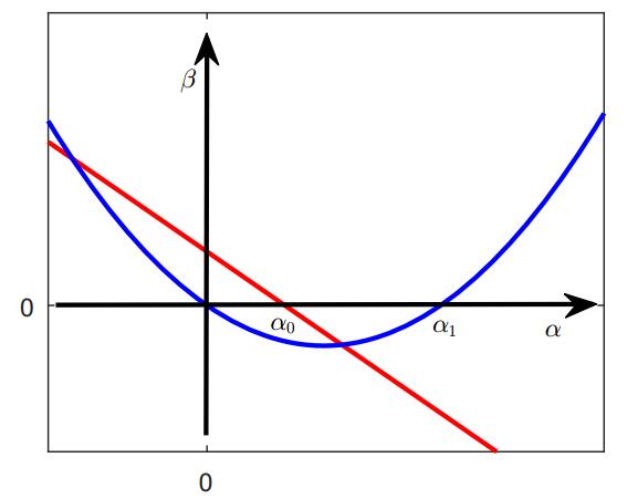
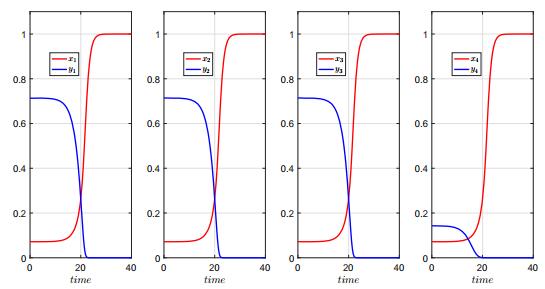
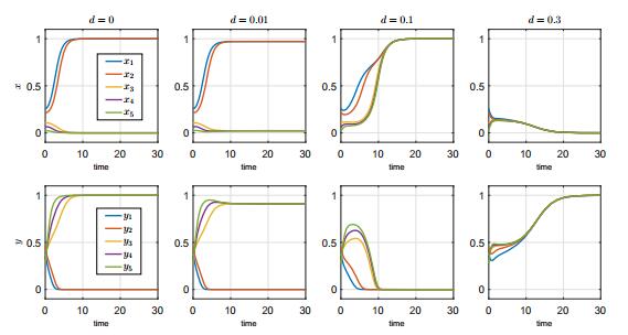
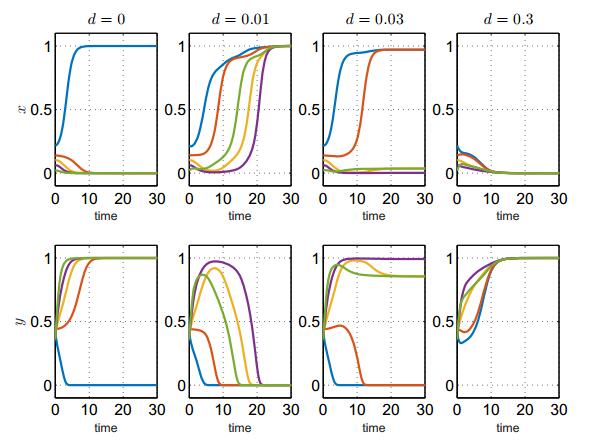
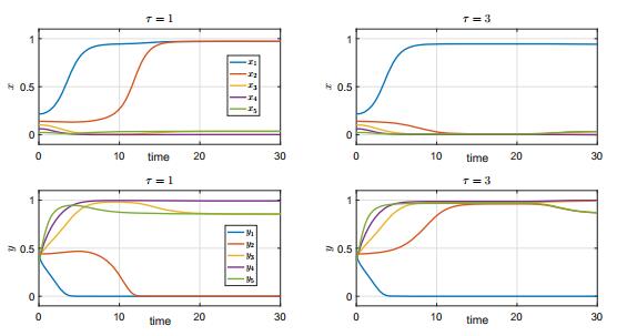
In this paper, we study a two-species competition model over patchy environments. One species is assumed to disperse randomly between patches with a constant dispersal delay. We show that the dispersal does not affect the stability and instability of the homogeneous coexistence equilibrium in two configurations (fully connected configuration and ring-structured configuration) of an arbitrary number of patches. For the weak competition case, we show that the homogeneous coexistence equilibrium is the unique coexistence equilibrium and both species can coexist. However, for the strong competition case, we show that the homogeneous coexistence equilibrium is unstable, in addition, small dispersal rate can induce multiple coexistence equilibria and the dispersal (including the dispersal rate and the dispersal delay) does have impacts on determining the competition outcome and can induce multi-stability. As a result, transient coexistence of both species can be observed in all patches, and long-term coexistence of both species in some patches, though not in all patches, becomes possible.
Citation: Ali Mai, Guowei Sun, Lin Wang. The impacts of dispersal on the competition outcome of multi-patch competition models[J]. Mathematical Biosciences and Engineering, 2019, 16(4): 2697-2716. doi: 10.3934/mbe.2019134
In this paper, we study a two-species competition model over patchy environments. One species is assumed to disperse randomly between patches with a constant dispersal delay. We show that the dispersal does not affect the stability and instability of the homogeneous coexistence equilibrium in two configurations (fully connected configuration and ring-structured configuration) of an arbitrary number of patches. For the weak competition case, we show that the homogeneous coexistence equilibrium is the unique coexistence equilibrium and both species can coexist. However, for the strong competition case, we show that the homogeneous coexistence equilibrium is unstable, in addition, small dispersal rate can induce multiple coexistence equilibria and the dispersal (including the dispersal rate and the dispersal delay) does have impacts on determining the competition outcome and can induce multi-stability. As a result, transient coexistence of both species can be observed in all patches, and long-term coexistence of both species in some patches, though not in all patches, becomes possible.

| [1] | I. Hanski, M. Gilpin and D. McCauley, Metapopulation Biology, Elsevier, 454 (1997). |
| [2] | R. Nathan and L. Giuggioli, A milestone for movement ecology research, Mov. Ecol., 1 (2013), 1–3. |
| [3] | M. Holyoak and S. Lawler, The role of dispersal in predator–prey metapopulation dynamics, J. Anim. Ecol., 65 (1996), 640–652. |
| [4] | C. Huff aker, Experimental studies on predation: dispersion factors and predator-prey oscillations, Hilgardia, 27 (1958), 343–383. |
| [5] | R. Holt, Population dynamics in two-patch environments: some anomalous consequences of an optimal habitat distribution, Theor. Popul. Biol., 28 (1985), 181–208. |
| [6] | K. Liao and Y. Lou, The eff ect of time delay in a two-patch model with random dispersal, Bull. Math. Biol., 76 (2014), 335–376. |
| [7] | W. Feng, B. Rock and J.Hinson, On a new model of two-patch predator prey system with migration of both species, J. Appl. Anal. Comput., 1(2011), 193–203. |
| [8] | H. Freedman and Y. Takeuchi, Global stability and predator dynamics in a model of prey dispersal in a patchy environment, Nonlinear Anal., 13 (1989), 993–1002. |
| [9] | C. Hauzy, M. Gauduchon, F. Hulot, et al., Density-dependent dispersal and relative dispersal aff ect the stability of predator–prey metacommunities, J. Theoret. Biol., 266 (2010), 458–469. |
| [10] | Y. Kang, K. Sourav and M. Komi, A two-patch prey-predator model with predator dispersal driven by the predation strength, Math. Biosci. Eng., 14 (2017), 843–880. |
| [11] | Y. Kuang and Y. Takeuchi, Predator-prey dynamics in models of prey dispersal in two-patch environments, Math. Biosci., 120 (1994), 77–98. |
| [12] | A. Mai, G. Sun and L. Wang, Impacts of the dispersal delay on the stability of the coexistence equilibrium of a two-patch predator-prey model with random predator dispersal, Bull. Math. Biol., (2019), doi.org/10.1007/s11538-018-00568-8. |
| [13] | A. Mai, G. Sun, F. Zhang, et al., The joint impacts of dispersal delay and dispersal patterns on the stability of predator-prey metacommunities, J. Theoret. Biol., 462 (2019), 455–465. |
| [14] | E. Matthysen, Density-dependent dispersal in birds and mammals, Ecography, 28 (2005), 403– 416. |
| [15] | R. Mchich, P. Auger and J. Poggiale, Eff ect of predator density dependent dispersal of prey on stability of a predator–prey system, Math. Biosci., 206 (2007), 343–356. |
| [16] | K. Messan and Y. Kang, A two patch prey-predator model with multiple foraging strategies in predator: Applications to insects, Discrete Contin. Dyn. Syst. Ser. B, 22 (2017), 947–976. |
| [17] | W. Wang and Y. Takeuchi, Adaptation of prey and predators between patches, J. Theoret. Biol., 258 (2009), 603–613. |
| [18] | Y. Zhang, F. Lutscher and F. Guichard, The eff ect of predator avoidance and travel time delay on the stability of predator-prey metacommunities, Theoret. Ecol., 8 (2015),273–283. |
| [19] | R. Cressman and V. Křivan, Two-patch population models with adaptive dispersal: the eff ects of varying dispersal speeds, J. Math. Biol., 67 (2013), 329–358. |
| [20] | X. Zhang and W. Wang, Importance of dispersal adaptations of two competitive populations between patches, Ecol. Model., 222 (2011), 11–20. |
| [21] | J. Murray, Mathematical Biology, New York: Springer-Verlag, (2002). |
| [22] | K. Cooke and Z. Grossman, Discrete delay, distributed delay and stability switches, J. Math. Anal. Appl., 86 (1982), 592–627. |
| [23] | J. Hale and S. M. Verduyn Lunel, Introduction to Functional Diff erential Equations, New York: Springer Science & Business Media, 99 (1993). |
| [24] | Y. Kuang, Delay Diff erential Equations: with Applications in Population Dynamics, New York: Academic Press, 191 (1993). |
| [25] | B. Friedman, Eigenvalues of composite matrices, Math. Proc. Cambridge Philos. Soc., 57 (1961), 37–49. |
Figures(5)

Ali Mai, Guowei Sun, Lin Wang. The impacts of dispersal on the competition outcome of multi-patch competition models[J]. Mathematical Biosciences and Engineering, 2019, 16(4): 2697-2716. doi: 10.3934/mbe.2019134


 DownLoad: