Known stoichiometric models of a two species producer-grazer ecosystem have either neglected spatial dynamics or failed to track free phosphorus in the media. In this paper we present a spatially heterogeneous model that tracks phosphorus content in the producer and free phosphorus in the media. We simulate our model numerically under various environmental conditions. Multiple equilibria, with bistability and deterministic extinction of the grazer, are possible here. In conditions that had been previously studied without tracking free phosphorus we find cases where qualitatively different behavior is observed. In particular under certain environmental conditions previous models predict stable equilibria where our model predicts stable limit cycles near the surface. Oscillatory dynamics can have consequences on the population densities, which may spend some time at low values throughout the cycles where they are in danger of stochastic extinction.
Citation: Md Masud Rana, Chandani Dissanayake, Lourdes Juan, Kevin R. Long, Angela Peace. Mechanistically derived spatially heterogeneous producer-grazer model subject to stoichiometric constraints[J]. Mathematical Biosciences and Engineering, 2019, 16(1): 222-233. doi: 10.3934/mbe.2019012
Related Papers:
[1]
Md Nazmul Hassan, Angela Peace .
Mechanistically derived Toxicant-mediated predator-prey model under Stoichiometric constraints. Mathematical Biosciences and Engineering, 2020, 17(1): 349-365.
doi: 10.3934/mbe.2020019
[2]
Md Nazmul Hassan, Kelsey Thompson, Gregory Mayer, Angela Peace .
Effect of Excess Food Nutrient on Producer-Grazer Model under Stoichiometric and Toxicological Constraints. Mathematical Biosciences and Engineering, 2019, 16(1): 150-167.
doi: 10.3934/mbe.2019008
[3]
Ming Chen, Meng Fan, Congbo Xie, Angela Peace, Hao Wang .
Stoichiometric food chain model on discrete time scale. Mathematical Biosciences and Engineering, 2019, 16(1): 101-118.
doi: 10.3934/mbe.2019005
[4]
Lina Hao, Meng Fan, Xin Wang .
Effects of nutrient enrichment on coevolution of a stoichiometric producer-grazer system. Mathematical Biosciences and Engineering, 2014, 11(4): 841-875.
doi: 10.3934/mbe.2014.11.841
[5]
Lale Asik, Jackson Kulik, Kevin Long, Angela Peace .
Dynamics of a stoichiometric producer-grazer system with seasonal effects on light level. Mathematical Biosciences and Engineering, 2019, 16(1): 501-515.
doi: 10.3934/mbe.2019023
[6]
Yang Kuang, Jef Huisman, James J. Elser .
Stoichiometric Plant-Herbivore Models and Their Interpretation. Mathematical Biosciences and Engineering, 2004, 1(2): 215-222.
doi: 10.3934/mbe.2004.1.215
[7]
Jitai Liang, Junjie Wei .
Lyapunov functional for virus infection model with diffusion and state-dependent delays. Mathematical Biosciences and Engineering, 2019, 16(2): 947-966.
doi: 10.3934/mbe.2019044
[8]
Guangyu Sui, Meng Fan, Irakli Loladze, Yang Kuang .
The dynamics of a stoichiometric plant-herbivore model and its discrete analog. Mathematical Biosciences and Engineering, 2007, 4(1): 29-46.
doi: 10.3934/mbe.2007.4.29
[9]
Nazanin Zaker, Christina A. Cobbold, Frithjof Lutscher .
The effect of landscape fragmentation on Turing-pattern formation. Mathematical Biosciences and Engineering, 2022, 19(3): 2506-2537.
doi: 10.3934/mbe.2022116
[10]
Ming Chen, Menglin Gong, Jimin Zhang, Lale Asik .
Comparison of dynamic behavior between continuous- and discrete-time models of intraguild predation. Mathematical Biosciences and Engineering, 2023, 20(7): 12750-12771.
doi: 10.3934/mbe.2023569
Abstract
Known stoichiometric models of a two species producer-grazer ecosystem have either neglected spatial dynamics or failed to track free phosphorus in the media. In this paper we present a spatially heterogeneous model that tracks phosphorus content in the producer and free phosphorus in the media. We simulate our model numerically under various environmental conditions. Multiple equilibria, with bistability and deterministic extinction of the grazer, are possible here. In conditions that had been previously studied without tracking free phosphorus we find cases where qualitatively different behavior is observed. In particular under certain environmental conditions previous models predict stable equilibria where our model predicts stable limit cycles near the surface. Oscillatory dynamics can have consequences on the population densities, which may spend some time at low values throughout the cycles where they are in danger of stochastic extinction.
1.
Introduction
Ecological stoichiometry studies how the balance of energy and elements affects and is affected by organisms and their interactions in ecosystems [2,16]. A stoichiometric model of producer-grazer interactions will necessarily consider both, food quantity and food quality since they determine the growth rate of consumers as well as their odds of survival and extinction [18].
In this paper we study the dynamics of a two species producer-grazer (algae-Daphnia) ecosystem when the essential nutrient phosphorus is tracked in both the producer and the media. Our main references are the LKE model developed by Loladze et al. [12], its spatial extension by Dissanayake [6] and an extension by Wang et al. [18]. The LKE is a two dimensional stoichiometric model where carbon is used to measure the biomass of the populations, and phosphorus is implicitly tracked through the phosphorus to carbon (P:C) ratio. The main model assumptions are:
A1: The total mass of phosphorus in the entire system is fixed, i.e., the system is closed for phosphorus with a total of P (mg P / L).
A2: P:C ratio in the producer varies, but it never falls below a minimum q (mg P / mg C); the grazers maintain constant P:C, θ (mg P / mg C).
A3: All phosphorus in the system is divided into two pools: phosphorus in the grazer and phosphorus in the producer.
The incorporation of chemical heterogeneity and stoichiometric constraints in the LKE model leads to complex dynamics with multiple equilibria, where bistability and deterministic extinction of the grazer are possible. This model highlights the important fact that energy enrichment of producer-grazer systems is dynamically different than nutrient enrichment.
Dissanayake [6] extended the LKE model to include spatial dynamics. The extended model still uses the three assumptions above and deals with the phosphorus in the same way as the LKE, only tracking it implicitly through the (P:C) ratios of the producer and consumer. The assumption A3 is also dropped in the spatially homogeneous model developed by Wang et al. [18], which extends the LKE to explicitly track phosphorus in the producer and the media. Such considerations result in a 4-D model which in their case leaves out consideration of spatial dynamics of the system. With diffusivity not present in their model, the sole verification that the total amount of phosphorus in the system is constant allows them to drop one equation and work with a reduced 3-D model.
In this paper our starting point is the spatial extension of the LKE model proposed by Dissanayake [6]. Then, similarly to Wang et al. [18], we arrive at a 4-D model mechanistically formulated to explicitly track phosphorus in the producer and the media. Since our model incorporates spatial dynamics, unlike [18], we do not reduce it down to a 3-D model. To make that work in a spatially heterogeneous model, we would need to add the rather unrealistic assumption that the diffusivities of all variables in the system are equal. In reality, Daphnia diffusivity is higher than the rest, and we choose to stay in the 4-D model.
Numerical simulations of our model reveal rich dynamics where the existence and stability of equilibria and limit cycles depend on depth. For model comparisons, we ran numerical simulations of a modified version of the model proposed by Dissanayake [6]. This allowed us to compare a spatial model that uses the above three assumptions with our model that drops assumption A3 and explicitly tracks free P in space. Under the same parameter sets, we observed qualitative differences between these two models, which highlight the importance of considering environmental nutrients loads in stoichiometric models.
2.
Model development
We begin with the spatially heterogeneous model developed in [6], where assumptions A1-A3 from [12] are kept. Let u be the biomass density of producer (algae) and v be the biomass density of grazer (Daphnia). The model is given by:
where Dz is the effective turbulent diffusivity; Du, the algal particle diffusivity; Dv, the Daphnia particle diffusivity; b, the algal maximum growth rate; Pt, the fixed total amount of phosphorus in the system; q, the minimum algal P:C ratio required for growth; θ, the constant P:C ratio of the Daphnia; ˆe, the Daphnia maximum conversion efficiency and d, the Daphnia loss rate. The spatial coordinate is represented by ˉx=(x,y,z), although in our analysis below we assume a one dimensional model that represents a water column with z as depth. The algal P:C ratio is denoted by Q and is defined as
Q=Pt−θvu,
where the quantity Pt−θv represents the available phosphorus for the algae. Note that this follows from assumption A3 above, as the P in the algae equals the total amount in the system, Pt, minus the P in the grazer population, θv.
In this model, K(z) represents the algae carrying capacity in terms of carbon, which is measured through the depth dependent irradiance discussed in Section 2.1 of this paper. The Daphnia biomass density is assumed to follow a Holling type Ⅱ functional response:
f(u)=cua+u
where a is the half saturation constant for grazer ingestion and c is the maximum ingestion rate.
Following Wang et al. [18], where P is tracked in a spatially homogeneous model, we drop assumption A3 and explicitly track the phosphorus in algae and free phosphorus in the media. Here, we now assume that all P in the system is divided into three pools: P in the grazer, P in the producer, and free P in the environment. Let Pa be the density of phosphorus in algae and Pf be the density of free phosphorus in the media. These P quantities depend on space and time. Our extended model takes the following form:
where Dp is the particle diffusivity of phosphorus and ˆd the loss rate of phosphorus for the producer. The algal P:C ratio Q in equation (2b) here takes the form
Q=Pau;
The phosphorus uptake rate of the producer is given by g(Pf) and is also assumed to follow a Holling type Ⅱ functional response:
g(Pf)=ˆcPfˆa+Pf.
Here ˆa is the phosphorus half saturation constant, and ˆc is the maximum phosphorus uptake rate of the algae population. The remaining parameters in Model (2) mean the same as in Model (1). The parameter values that we use in the numerical simulations are given in Table 1.
Free phosphorus occurs in many forms in our system, including phosphorus ions and phosphorus bound in dead organisms and macromolecular metabolic waste. Typical diffusion coefficients for atoms, ions, and small molecules in water are on order 10−5cm2s−1[4], which in our units is 8.64×10⁻⁵m2day−1. We adopt a nominal value of 10−4m2day−1 for Dp; note that this is identical to our choice of algal diffusivity Du.
The domain of our one-dimensional model is [0,H] with the water's surface at z=0 and H is the total depth of the water column in meters. At both boundaries, no-flux conditions hold for both populations and P quantities.
−(Dz+Du)∂u∂z=0,−(Dz+Dv)∂v∂z=0,−(Dz+Du)∂Pa∂z=0, and −(Dz+Dp)∂Pf∂z=0
Thus the total phosphorus in system (2) remains constant at all time. In the special case where the four variables u,v,Pa and Pf have exactly the same diffusivity, the global constraint (5) implies the local constraint Pt=Pf+Pa+θv which can be used to reduce the 4-D Model (2) to a 3-D model as in [18]. However, that is not a realistic assumption since in the real world Daphnia diffusivity is higher than the diffusivity of the other variables in the system. Here, we consider the 4-D Model (2) with the global constraint given by equation (5).
2.1. Light absorption
In a 1-dimensional medium, the irradiance I obeys the equation of radiative transfer [9,15],
dIdz=−κI
(6)
with boundary condition at the surface
I(0)=I0
(7)
where κ denotes the absorption coefficient and I0 is the irradiance at the surface. In cases where κ is a constant, the familiar Lambert-Beer's exponential law I(z)=I0exp(−κz) is recovered. In an aquatic ecosystem, the light is absorbed by the water molecules, dissolved organic matter, phytoplankton population and many other light absorbing substances [8,9]. Thus, we assume the absorption coefficient depends on the density of the phytoplankton population as
κ(u)=κuu+κbg
(8)
where κu is the specific light attenuation coefficient of algal biomass and κbg is the total background turbidity due to non-phytoplankton components.
Irradiance is an important factor for the producer's carrying capacity, when producer growth is limited by carbon. The LKE model assumes K0 is positively correlated with irradiance. Given a particular irradiance and ample nutrients, the producer density grows but eventually stabilizes at K0 due to shelf-shading. In our extended model the irradiance varies with depth following Equation (6). Here, we assume a linear relationship between the irradiance and carbon-dependent producer carrying capacity K,
K(z)=αI(z)
(9)
where α is a conversion coefficient correlating irradiance with the producer carrying capacity, under environmental conditions where growth is limited by light-supplied carbon. The largest carrying capacity will occur on the surface where irradiance is the largest I0. Non-spatial stoichiometric models typically assume algal carrying capacity K0∈(0,3) mg C/L. In order to relate to these models and stay within similar parameter space we assume the irradiance at the surface, I0 corresponds to K(0)=K0 and parameterize α accordingly. Given that global average irradiance is 1,366 watts/m2[9], We assume α = 1.098 mg C/m/watts and consider values K0∈(0,3) mg C/L.
3.
Numerical methods
We conduct series of numerical experiments of Model (1) and Model (2) in order to understand the population dynamics under various environmental conditions. The parameters values are summarized in Table 1.
The reaction-advection diffusion equation Model (1) and Model (2) together with equation (6) for radiative transport, form a system of nonlinear partial differential equations which must be solved numerically. Our simulation methods are based on those developed by Dissanayake [6] for an algae-daphnia ecosystem with stoichiometry and diffusion, which were then further extended in Dissanayake at al. [7]. The reader is referred to [7] for a fuller description of the numerical methods used.
4.
Results
Numerical simulations of model (2) are presented in Figures 1 and 2 for varying levels of light K0 and two concentrations of total phosphorus Pt. The simulations represent a one dimensional water column with a depth of 20 meters. Surface plots for the algae producer population density for varying time and depth are shown in Figure 1. Under low light conditions corresponding to a low surface algae carrying capacity K0=0.5 mg C/L the population exist at a stable equilibria which decreases with depth (Figure 1(a)). Under higher light conditions corresponding to a higher surface algae carrying capacity K0=1 mg C/L the population exhibits oscillations near the surface, which dampen to stable equilibria as depth increases (Figure 1(b)).
Figure 1.
Numerical simulations of the producer population density for Model (2) for K0=0.5 mg C/L (a) and K0=1.0 mg C/L (b) and intermediate Pt=0.6 mg P.
Figure 2.
Numerical simulation snap shots for a fixed time showing steady-state behavior for Model (2) for intermediate Pt=0.6 mgP (a), (c), (e) and high Pt=1.0 mgP (b), (d), (f). The surface light levels is also varied: K0=0.5 mg C/L (a)-(b), K0=1.0 mg C/L (c)-(d), and K0=2.0 mg C/L (e)-(f). The horizontal axis is depth in meters, so highest light levels occur on the left at the surface. Regions where solutions exhibit sustained oscillations are shaded in gray. Unshaded regions depict equilibrium solutions.
Figure 2 show snapshots of these dynamics for a single time point showing steady state behaviors for varying depths. The curves represent stable equilibria and stable limit cycles. The first column of figures considers intermediate values of Pt=0.6 mg P, which corresponds to 0.03 mg P/L. The second column of figures considers high values of Pt=1.0 mg P, which correspond to 0.05 mg P/L. The unshaded regions in these figures depict the solutions of the model at equilibria and the shaded regions depict regions with stable limit cycles.
Population dynamics depend on the level of light at the surface. For a low light level at the surface corresponding with a low producer carrying capacity K0=0.5 mg C/L the model predicts stable equilibria solutions throughout the entire water column for both levels of P, see Figures 2a and b. The algae and Daphnia population coexist near the surface. As depth increases, eventually the Daphnia population dies out, near six meters for both P levels. The algal P:C ratio, Q is lowest near the surface, where the level of light is highest. Comparing Figure 2a with Figure 2b, we see that Q is higher under higher Pt, however the algae and Daphnia population dynamics are similar. Here, both populations are limited by C, and growth is not limited by P. For K0=0.5 mg C/L Daphnia is limited by food quantity.
For intermediate light levels at the surface corresponding with producer carrying capacity K0=1 mg C/L the model exhibits sustained oscillatory dynamics near the surface and stable equilibria solutions at low depths for both Pt conditions, see Figures 2c and d. As depth increases, the stable limit cycles collapse between six and seven meters. Here, the Daphnia are able to persist at deeper depth than the low light predictions.
Under high light levels at the surface corresponding with producer carrying capacity K0=2 mg C/L the model exhibits stable equilibria throughout the entire water column under intermediate Pt=0.6 mg P conditions, see Figure 2e. The equilibria observed near the surface consist of high algae densities but constrained Daphnia densities. These constrained grazer densities are due to stoichiometric constraints, as the P:C ratio of algae near the surface is low. Algae near the surface are exposed to high light levels and therefore make low quality food for the grazer. On the other hand, stable equilibria observed at lower depths consist of lower algae densities of higher quality, high Q. At these lower depths, despite the lower food quantity the Daphnia population survives due to high food quality. At very low depths algal densities become low enough, the Daphnia become limited by food quantity again. As depth continues to increase, eventually the Daphnia population dies out, near 10 meters.
While the model predicts stable equilibria throughout the entire water column under high light levels for intermediate P levels, under high light and high Pt=1.0 mg P conditions, the model exhibits stable limit cycles near the surface, see Figure 2f. Near the surface, the Daphnia population obtains very high densities during the oscillatory dynamics. The limit cycles have large amplitude. Throughout these oscillations, it is likely that Daphnia experience both C and P limitations, as both food quality and quantity oscillate. Comparing the region of oscillations (shaded regions in Figure 2c, d and f.), we can see that under high light levels the oscillations persist to deeper depth.
5.
Discussion
We developed a stoichiometric producer-grazer model that explicitly tracks the quantity and the nutritional quality of the producer in time and space. The model is formulated by mechanistically accounting for the content of two essential elements C and P as they vary with depth. The developed model is an extension of the spatial stoichiometric producer-grazer model by Dissanayake [6], which assumes algal is extremely efficient at taking up nutrients. Here, we explicitly track free P in the environment. Numerical simulations yield rich dynamics where the existence and stability of equilibria and limit cycles depend on depth (Figures 1 and 2).
In order to investigate the impact of tracking free P we compare numerical simulations of two stoichiometric spatially heterogeneous models, Model (1) developed by Dissanayake [6] with our modification of light absorption, and our extension which explicitly tracks environmental P, Model (2). Figures 3 and 4 present a comparison between Model (1) and Model (2). The parameter values for light and P used in these simulations are examples where the two models predict qualitatively different dynamics. Here, for Model (2) we set Pt to correspond with the same level of total P used in Model (1). Under high light K0=1.5 mg C/L and intermediate levels of total P=0.03 mg P/L Model (1) predicts stable equilibria throughout the entire water column, however Model (2) exhibits stable limit cycles near the surface and stable equilibria at lower depths, see Figure 3. Interestingly, under very high light K0=2.5 mg C/L and slightly higher intermediate level of total P=0.035 mg P/L the behavior of the predicted population dynamics switches between the two models, see Figure 4. Under these parameter conditions, Model (1) now exhibits sustained oscillatory dynamics near the surface, whereas Model (2) has stable equilibria throughout the entire water column. Figures 3 and 4 are two example regions in parameter space where our Model (2) has qualitatively different dynamics than previous models that neglect to track environmental P loads.
Figure 3.
Numerical simulations snap shots for a fixed time showing steady-state behavior for Model (1) (a) and Model (2) (b) for K0=1.5 mg C/L and P=0.03 mg P/L. Regions where solutions exhibit sustained oscillations are shaded in gray. Unshaded regions depict equilibrium solutions.
Figure 4.
Numerical simulations snap shots for a fixed time showing steady-state behavior for Model (1) (a) and Model (2) (b) for K0=2.5 mg C/L and P=0.035 mg P/L. Regions where solutions exhibit sustained oscillations are shaded in gray. Unshaded regions depict equilibrium solutions.
The discrepancies between the predictions of these two models can have important implications. Under certain environmental conditions the previous model that incorporate spatial dynamics but neglect to track aquatic free P predict stable equilibria when our model predicts stable limit cycles near the surface. Here the grazer Daphnia population densities can get to low values during the oscillations, where they are in danger of stochastic extinction (Figure 3). During these oscillatory dynamics the amplitudes of the oscillations become important to avoid possible extinction.
Interestingly, under very high light the previous spatial model that neglects to track aquatic free P predicts limit cycles near the surface where our model predicts the existence of stable equilibria (Figure 4). Further investigations into these discrepancies should be conducted. We hypothesize that the dynamics are sensitive to the resource limitation switch Daphnia experience, where they're growth is either nutrient or light limited.
These types of qualitative differences are also seen in the absence of spatial dynamics. Wang et al. [18] demonstrated that explicitly tracking free nutrients in spatially homogeneous stoichiometric models can yield qualitatively different dynamics than spatially homogeneous models that don't allow for the environmental nutrient load. Peace et al. [14] also investigated the effects of explicitly tracking free nutrients in a model that considers the consequences of excess nutrients as well nutrient limitations. Mechanistically formulated models that track free nutrients, like Model (2) and the models presented in Wang et al. [18] and Peace et al. [14] can be easily expanded to multiple producers and grazers while maintaining their structure.
It is important to note that in this manuscript we considered simplified dynamics for particle transport and focused our efforts on exploring the effects of stoichiometric constraints on population dynamics over space and time. Future enhancements to the model should include buoyancy, as plankton can self-regulate buoyancy to seek nutrients or light.
Acknowledgments
Peace is supported by NSF grant DMS - 1615697.
Conflict of interest
The authors declare there is no conflicts of interest.
References
[1]
T. Andersen (1997) Pelagic nutrient cycles; herbivores as sources and sinks. Springer, Berlin.
[2]
T. Andersen , J. J. Elser and D. O. Hessen, Stoichiometry and population dynamics. Ecol. Lett., 7 (2004), 884–900.
[3]
S. A. Berger, S. Diehl, T. J. Kunz, D. Albrecht, A. M. Oucible and S. Ritzer, Light supply, plankton biomass, and seston stoichiometry in a gradient of lake mixing depths. Limnol. Oceanogr., 51 (2006), 1898–1905.
[4]
E. L. Cussler (1996) Diffusion: Mass Transfer in Fluid Systems. Cambridge University Press.
[5]
S. Diehl, S. Berger and R. W¨ohrl, Flexible nutrient stoichiometry mediates environmental influences on phytoplankton and its resources. Ecology , 86 (2005), 2931–2945.
[6]
C. Dissanayake (2016) Finite element simulation of space/time behavior in a two species ecological stoichiometric model. PhD thesis, Texas Tech University.
[7]
C. Dissanayake, L. Juan, K. R. Long, A. Peace and M. M. Rana (under review 2018) Genotypic selection in spatially heterogeneous producer-grazer systems subject to stoichiometric constraints. Bulletin of Mathematical Biology.
[8]
J. Huisman, J. Sharples, J. M. Stroom, P. M. Visser, W. E. A. Kardinaal, J. M. Verspagen and Sommeijer B, Changes in turbulent mixing shift competition for light between phytoplankton species. Ecology, 85 (2004), 2960–2970.
[9]
J. T. Kirk (1994) Light and photosynthesis in aquatic ecosystems. Cambridge University Press.
[10]
D. Kuefler, T. Avgar and J. M. Fryxell, Rotifer population spread in relation to food, density and predation risk in an experimental system. J. Anim. Ecol., 81 (2012), 323–329.
[11]
D. Kuefler, T. Avgar and J. M. Fryxell, Density-and resource-dependent movement characteristics in a rotifer. Funct. Ecol., 27 (2013), 323–328.
[12]
I. Loladze, Y. Kuang and J. J. Elser, Stoichiometry in producer–grazer systems: linking energy flow with element cycling. Bull. Math. Biol., 62 (2000), 1137–1162.
[13]
A. Lorke, Investigation of turbulent mixing in shallow lakes using temperature microstructure measurements. Aquat. Sci.-Research Across Boundaries, 60 (1998), 210–219.
[14]
A. Peace, H.Wang and Y. Kuang, Dynamics of a producer–grazer model incorporating the effects of excess food nutrient content on grazer's growth. Bull. Math. Biol., 76 (2014), 2175–2197.
[15]
F. H. Shu (1991) The Physics of Astrophysics, Vol. 2: Radiation. Univ. Sci. Books, Mill Valley CA.
[16]
R. W. Sterner and J. J. Elser (2002) Ecological stoichiometry: the biology of elements from molecules to the biosphere. Princeton University Press.
[17]
H. Wang, H. L. Smith, Y. Kuang and J. J. Elser, Dynamics of stoichiometric bacteria-algae interactions in the epilimnion. SIAM J. Appl. Math., 68 (2007), 503–522.
[18]
H. Wang, Y. Kuang and I. Loladze, Dynamics of a mechanistically derived stoichiometric producer-grazer model. J. Biol. Dynam., 2 (2008), 286–296.
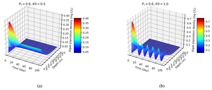
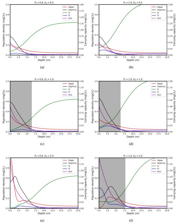
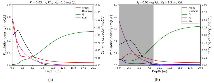
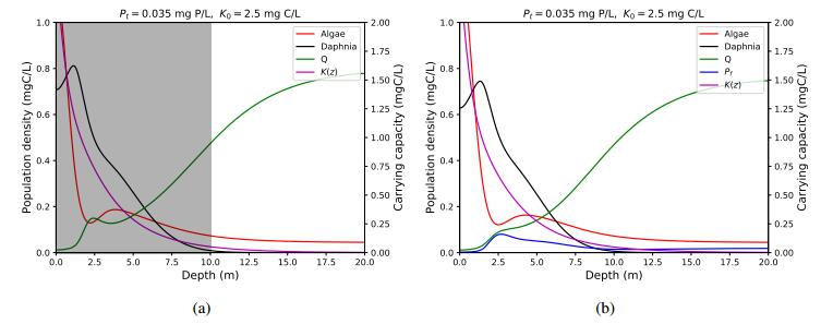
This article has been cited by:
1.
Simran Kaur Sandhu, Andrew Morozov, Lourdes Juan,
Exploring the role of spatial and stoichiometric heterogeneity in the top-down control in eutrophic planktonic ecosystems,
2020,
499,
00225193,
110311,
10.1016/j.jtbi.2020.110311
2.
Chandani Dissanayake, Lourdes Juan, Kevin R. Long, Angela Peace, Md Masud Rana,
Genotypic Selection in Spatially Heterogeneous Producer-Grazer Systems Subject to Stoichiometric Constraints,
2019,
81,
0092-8240,
4726,
10.1007/s11538-018-00559-9
3.
Angela Peace, Paul C Frost, Nicole D Wagner, Michael Danger, Chiara Accolla, Philipp Antczak, Bryan W Brooks, David M Costello, Rebecca A Everett, Kevin B Flores, Christopher M Heggerud, Roxanne Karimi, Yun Kang, Yang Kuang, James H Larson, Teresa Mathews, Gregory D Mayer, Justin N Murdock, Cheryl A Murphy, Roger M Nisbet, Laure Pecquerie, Nathan Pollesch, Erica M Rutter, Kimberly L Schulz, J Thad Scott, Louise Stevenson, Hao Wang,
Stoichiometric Ecotoxicology for a Multisubstance World,
2021,
71,
0006-3568,
132,
10.1093/biosci/biaa160
4.
Tianxu Wang, Hao Wang,
Stoichiometric microplastics models in natural and laboratory environments,
2024,
580,
00225193,
111733,
10.1016/j.jtbi.2024.111733
5.
Tianxu Wang, Hao Wang,
Stoichiometry-Dependent Fear Effect in a Food Chain Model,
2024,
84,
0036-1399,
783,
10.1137/23M1581613
Figure 1. Numerical simulations of the producer population density for Model (2) for K0=0.5 mg C/L (a) and K0=1.0 mg C/L (b) and intermediate Pt=0.6 mg P
Figure 2. Numerical simulation snap shots for a fixed time showing steady-state behavior for Model (2) for intermediate Pt=0.6 mgP (a), (c), (e) and high Pt=1.0 mgP (b), (d), (f). The surface light levels is also varied: K0=0.5 mg C/L (a)-(b), K0=1.0 mg C/L (c)-(d), and K0=2.0 mg C/L (e)-(f). The horizontal axis is depth in meters, so highest light levels occur on the left at the surface. Regions where solutions exhibit sustained oscillations are shaded in gray. Unshaded regions depict equilibrium solutions
Figure 3. Numerical simulations snap shots for a fixed time showing steady-state behavior for Model (1) (a) and Model (2) (b) for K0=1.5 mg C/L and P=0.03 mg P/L. Regions where solutions exhibit sustained oscillations are shaded in gray. Unshaded regions depict equilibrium solutions
Figure 4. Numerical simulations snap shots for a fixed time showing steady-state behavior for Model (1) (a) and Model (2) (b) for K0=2.5 mg C/L and P=0.035 mg P/L. Regions where solutions exhibit sustained oscillations are shaded in gray. Unshaded regions depict equilibrium solutions