Currently, the discrete Hopfield neural network deals with challenges related to searching space and limited memory capacity. To address this issue, we propose integrating logical rules into the neural network to regulate neuron connections. This approach requires adopting a specific logic framework that ensures the network consistently reaches the lowest global energy state. In this context, a novel logic called major 1,3 satisfiability was introduced. This logic places a higher emphasis on third-order clauses compared to first-order clauses. The proposed logic is trained by the exhaustive search algorithm, aiming to minimize the cost function toward zero. To evaluate the proposed model effectiveness, we compare the model's learning and retrieval errors with those of the existing non-systematic logical structure, which primarily relies on first-order clauses. The similarity index measures the similarity benchmark neuron state with the existing and proposed model through extensive simulation studies. Certainly, the major random 1,3 satisfiability model exhibited a more extensive solution space when the ratio of third-order clauses exceeds 0.7% compared to first-order clauses. As we compared the experimental results with other state-of-the-art models, it became evident that the proposed model achieved significant results in capturing the overall neuron state. These findings emphasize the notable enhancements in the performance and capabilities of the discrete Hopfield neural network.
Citation: Gaeithry Manoharam, Azleena Mohd Kassim, Suad Abdeen, Mohd Shareduwan Mohd Kasihmuddin, Nur 'Afifah Rusdi, Nurul Atiqah Romli, Nur Ezlin Zamri, Mohd. Asyraf Mansor. Special major 1, 3 satisfiability logic in discrete Hopfield neural networks[J]. AIMS Mathematics, 2024, 9(5): 12090-12127. doi: 10.3934/math.2024591
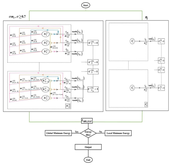
Currently, the discrete Hopfield neural network deals with challenges related to searching space and limited memory capacity. To address this issue, we propose integrating logical rules into the neural network to regulate neuron connections. This approach requires adopting a specific logic framework that ensures the network consistently reaches the lowest global energy state. In this context, a novel logic called major 1,3 satisfiability was introduced. This logic places a higher emphasis on third-order clauses compared to first-order clauses. The proposed logic is trained by the exhaustive search algorithm, aiming to minimize the cost function toward zero. To evaluate the proposed model effectiveness, we compare the model's learning and retrieval errors with those of the existing non-systematic logical structure, which primarily relies on first-order clauses. The similarity index measures the similarity benchmark neuron state with the existing and proposed model through extensive simulation studies. Certainly, the major random 1,3 satisfiability model exhibited a more extensive solution space when the ratio of third-order clauses exceeds 0.7% compared to first-order clauses. As we compared the experimental results with other state-of-the-art models, it became evident that the proposed model achieved significant results in capturing the overall neuron state. These findings emphasize the notable enhancements in the performance and capabilities of the discrete Hopfield neural network.

| [1] |
M Soori, B. Arezoo, R. Dastres, Artificial intelligence, machine learning and deep learning in advanced robotics, Cognit. Rob. , 3 (2023), 54–70.https://doi.org/10.1016/j.cogr.2023.04.001 doi: 10.1016/j.cogr.2023.04.001

|
| [2] |
J. L. Patel, R. K. Goyal, Applications of artificial neural networks in medical science, Curr. Clin. Pharmacol. , 2 (2007), 217–226.https://doi.org/10.2174/157488407781668811 doi: 10.2174/157488407781668811
|
| [3] |
L. Feng, J. Zhang, Application of artificial neural networks in tendency forecasting of economic growth, Econ. Modell. , 40 (2014), 76–80.https://doi.org/10.1016/j.econmod.2014.03.024 doi: 10.1016/j.econmod.2014.03.024
|
| [4] |
A. Nikitas, K. Michalakopoulou, E. T. Njoya, D. Karampatzakis, Artificial intelligence, transport and the smart city: definitions and dimensions of a new mobility era, Sustainability, 12 (2020), 2789.https://doi.org/10.3390/su12072789 doi: 10.3390/su12072789
|
| [5] |
M. Ozbey, M. Kayri, Investigation of factors affecting transactional distance in E-learning environment with artificial neural networks, Educ. Inf. Technol. , 28 (2023), 4399–4427.https://doi.org/10.1007/s10639-022-11346-4 doi: 10.1007/s10639-022-11346-4
|
| [6] |
M. Tkac, R. Verner, Artificial neural networks in business: two decades of research, Appl. Soft Comput. , 38 (2016), 788–804.https://doi.org/10.1016/j.asoc.2015.09.040 doi: 10.1016/j.asoc.2015.09.040
|
| [7] | N. J. Nilsson, Probabilistic logic, Artif. Intell. , 28 (1986), 71–87. |
| [8] |
C. Nebauer, Evaluation of convolutional neural networks for visual recognition, IEEE Trans. Neual Networks, 9 (1998), 685–696.https://doi.org/10.1109/72.701181 doi: 10.1109/72.701181
|
| [9] | D. O. Hebb, The organization of behavior: a neuropsychological theory, John Wiley and Sons, Inc, 1949. |
| [10] |
S. F. Ahmed, M. S. B. Alam, M. Hassan, Deep learning modelling techniques: current progress, applications, advantages, and challenges, Artif. Intell. Rev. , 56 (2023), 13521–13617.https://doi.org/10.1007/s10462-023-10466-8 doi: 10.1007/s10462-023-10466-8
|
| [11] | S. Sathasivam, Upgrading logic programming in Hopfield network, Sains Malays. , 39 (2010), 115–118. |
| [12] |
S. Sathasivam, W. A. T. W. Abdullah, Logic mining in neural network: reverse analysis method, Computing, 91 (2011), 119–133.https://doi.org/10.1007/s00607-010-0117-9 doi: 10.1007/s00607-010-0117-9
|
| [13] |
W. A. T. W. Abdullah, Logic programming on a neural network, Int. J. Intell. Syst. , 7 (1992), 513–519.https://doi.org/10.1002/int.4550070604 doi: 10.1002/int.4550070604
|
| [14] | M. A. Mansor, S. Sathasivam, Optimal performance evaluation metrics for satisfiability logic representation in discrete Hopfield neural network, Comput. Sci. , 16 (2021), 963–976. |
| [15] |
M. A. Mansor, M. S. M. Kasihmuddin, S. Sathasivam, Robust artificial immune system in the Hopfield network for maximum k-satisfiability, Int. J. Interact. Multimedia Artif. Intell., 4 (2017), 63.https://doi.org/10.9781/ijimai.2017.448 doi: 10.9781/ijimai.2017.448
|
| [16] |
M. S. M. Kasihmuddin, M. A. Mansor, S. Sathasivam, Discrete Hopfield neural network in restricted maximum k-satisfiability logic programming, Sains Malays. , 47 (2018), 1327–1335.https://doi.org/10.17576/JSM-2018-4706-30 doi: 10.17576/JSM-2018-4706-30
|
| [17] |
N. E. Zamri, M. A. Mansor, M. S. M. Kasihmuddin, A. Alway, M. S. Z. Jamaludin, S. A. Alzaeemi, Amazon employees resources access data extraction via clonal selection algorithm and logic mining approach, Entropy, 22 (2020), 596.https://doi.org/10.3390/e22060596 doi: 10.3390/e22060596
|
| [18] |
M. S. M. Kasihmuddin, M. A. Mansor, M. F. M. Basir, S. Sathasivam, Discrete mutation Hopfield neural network in propositional satisfiability, Mathematics, 7 (2019), 1133.https://doi.org/10.3390/math7111133 doi: 10.3390/math7111133
|
| [19] | M. S. M. Kasihmuddin, M. A. Mansor, S. Sathasivam, Hybrid genetic algorithm in the Hopfield neural network for logic satisfiability problem, Pertanika J. Sci. Technol., 25 (2017), 139152. |
| [20] |
S. Sathasivam, M. A. Mansor, A. I. M. Ismail, S. Z. M Jamaludin, M. S. M. Kasihmuddin, M. Mamat, Novel random k satisfiability for k≤2 in Hopfield neural network, Sains Malays. , 49 (2020), 2847–2857.https://doi.org/10.17576/jsm-2020-4911-23 doi: 10.17576/jsm-2020-4911-23
|
| [21] |
N. E. Zamri, S. A. Azhar, M. A. Mansor, A. Alway, M. S. M. Kasihmuddin, Weighted random k satisfiability for k = 1, 2 (r2SAT) in discrete Hopfield neural network, Appl. Soft Comput. , 126 (2022), 109312.https://doi.org/10.1016/j.asoc.2022.109312 doi: 10.1016/j.asoc.2022.109312
|
| [22] |
S. A. Karim, N. E. Zamri, A. Alway, M. S. M. Kasihmuddin, A. I. M. Ismail, M. A. Mansor, et al., Random satisfiability: a higher-order logical approach in discrete Hopfield neural network, IEEE Access, 9 (2021), 50831–50845.https://doi.org/10.1109/ACCESS.2021.3068998 doi: 10.1109/ACCESS.2021.3068998
|
| [23] |
M. M. Bazuhair, S. Z. M. Jamaludin, N. E Zamri, M. S. M. Kasihmuddin, M. Mansor, A. Alway, et al., Novel Hopfield neural network model with election algorithm for random 3 satisfiability, Processes, 9 (2021), 1292.https://doi.org/10.3390/pr9081292 doi: 10.3390/pr9081292
|
| [24] |
S. Sathasivam, M. A. Mansor, M. S. M. Kasihmuddin, H. Abubakar, Election algorithm for random k satisfiability in the Hopfield neural network, Processes, 8 (2020), 568.https://doi.org/10.3390/pr8050568 doi: 10.3390/pr8050568
|
| [25] |
A. Alway, N. E. Zamri, S. A. Karim, M. A. Mansor, M. S. M. Kasihmuddin, M. M. Bazuhair, Major 2 satisfiability logic in discrete Hopfield neural network, Int. J. Comput. Math. , 99 (2022), 924–948.https://doi.org/10.1080/00207160.2021.1939870 doi: 10.1080/00207160.2021.1939870
|
| [26] |
Y. Guo, M. S. M. Kasihmuddin, Y. Gao, M. A. Mansor, H. A. Wahab, N. E. Zamri, et al., YRAN2SAT: a novel flexible random satisfiability logical rule in discrete Hopfield neural nework, Adv. Eng. Software, 171 (2022), 103169.https://doi.org/10.1016/j.advengsoft.2022.103169 doi: 10.1016/j.advengsoft.2022.103169
|
| [27] | Y. Gao, Y. Guo, N. A. Romli, M. S. M. Kasihmuddin, W. Chen, M. A. Mansor, et al., GRAN3SAT: creating flexible higher-order logic satisfiability in the discrete Hopfield neural network, Mathematics, 10 (2022), 1899. https: /doi. org/10.3390/math10111899 |
| [28] |
S. Abdeen, M. S. M. Kasihmuddin, N. E. Zamri, G. Manoharam, M. A. Mansor, N. Alshehri, S-type random k satisfiability logic in discrete Hopfield neural network using probability distribution: performance optimization and analysis, Mathematics, 11 (2023), 984.https://doi.org/10.3390/math11040984 doi: 10.3390/math11040984
|
| [29] |
M. A. F. Roslan, N. E. Zamri, M. A. Mansor, M. S. M. Kasihmuddin, Major 3 satisfiability logic in discrete Hopfield neural network integrated with multi-objective election algorithm, AIMS Math. , 8 (2023), 22447–22482.https://doi.org/10.3934/math.20231145 doi: 10.3934/math.20231145
|
| [30] |
S. A. Karim, M. S. M. Kasihmuddin, S. Sathasivam, M. A. Mansor, S. Z. M. Jamaludin, M. R. Amin, A novel multi-objective hybrid election algorithm for higher-order random satisfiability in discrete Hopfield neural network, Mathematics, 10 (2022), 1963.https://doi.org/10.3390/math10121963 doi: 10.3390/math10121963
|
| [31] |
T. Fukai, S. Tanaka, A simple neural network exhibiting selective activation of neuronal ensembles: from winner-take-all to winners-share-all, Neural Comput. , 9 (1997), 77–97.https://doi.org/10.1162/neco.1997.9.1.77 doi: 10.1162/neco.1997.9.1.77
|
| [32] |
M. S. M. Kasihmuddin, S. Z. M. Jamaludin, M. A. Mansor, H. A. Wahab, S. M. S. Ghadzi, Supervised learning perspective in logic mining, Mathematics, 10 (2022), 915.https://doi.org/10.3390/math10060915 doi: 10.3390/math10060915
|
| [33] |
O. I. Abiodun, A. Jantan, A. E. Omolara, K. V. Dada, N. A. Mohamed, H. Arshad, State-of-the-art in artificial neural network applications: a survey, Heliyon, 4 (2018), e00938.https://doi.org/10.1016/j.heliyon.2018.e00938 doi: 10.1016/j.heliyon.2018.e00938
|
| [34] |
C. J. Willmott, K. Matsuura, Advantages of the mean absolute error (MAE) over the root mean square error (RMSE) in assessing average model performance, Climate Res. , 30 (2005), 79–82.https://doi.org/10.3354/CR030079 doi: 10.3354/CR030079
|
| [35] |
A. de Myttenaere, B. Golden, B. L. Grand, F. Rossi, Mean absolute percentage error for regression models, Neurocomputing, 192 (2016), 38–48.https://doi.org/10.1016/j.neucom.2015.12.114 doi: 10.1016/j.neucom.2015.12.114
|
| [36] |
M. Bilal, S. Masud, S. Athar, FPGA design for statistics-inspired approximate sum-of-squared-error computation in multimedia applications, IEEE Trans. Circuits Syst. II, 59 (2012), 506–510.https://doi.org/10.1109/TCSII.2012.2204841 doi: 10.1109/TCSII.2012.2204841
|
| [37] |
P. Ong, Z. Zainuddin, Optimizing wavelet neural networks using modified cuckoo search for multi-step ahead chaotic time series prediction, Appl. Soft Comput. , 80 (2019), 374–386.https://doi.org/10.1016/j.asoc.2019.04.016 doi: 10.1016/j.asoc.2019.04.016
|
| [38] |
P. Bergmann, K. Batzner, M. Fauser, D. Sattlegger, C. Steger, The MVTec anomaly detection dataset: a comprehensive real-world dataset for unsupervised anomaly detection, Int. J. Comput. Vision, 129 (2021), 1038–1059.https://doi.org/10.1007/s11263-020-01400-4 doi: 10.1007/s11263-020-01400-4
|
| [39] |
V. Lopez, A. Fernandez, S. Garcia, V. Palade, F. Herrera, An insight into classification with imbalanced data: empirical results and current trends on using data intrinsic characteristics, Inf. Sci. , 250 (2013), 113–141.https://doi.org/10.1016/j.ins.2013.07.007 doi: 10.1016/j.ins.2013.07.007
|
| [40] |
B. H. Goh, Forecasting residential construction demand in Singapore: a comparative study of the accuracy of time series, regression, and artificial neural network techniques, Eng. Constr. Archit. Manage. , 5 (1998), 261–275.https://doi.org/10.1046/j.1365-232X.1998.00048.x doi: 10.1046/j.1365-232X.1998.00048.x
|
| [41] |
J. J. Hopfield, Neural networks and physical systems with emergent collective computational abilities, Proc. Natl. Acad. Sci. , 79 (1982), 2554–2558.https://doi.org/10.1073/pnas.79.8.2554 doi: 10.1073/pnas.79.8.2554
|
| [42] |
V. Veerasamy, N. I. A. Wahab, R. Ramachandran, M. L. Othman, H. Hizam, A. X. R. Irudayaraj, et al., A Hankel matrix based reduced order model for stability analysis of hybrid power system using PSO-GSA optimized cascade PI-PD controller for automatic load frequency control, IEEE Access, 8 (2020), 71422–71446.https://doi.org/10.1109/ACCESS.2020.2987387 doi: 10.1109/ACCESS.2020.2987387
|
| [43] |
X. Fan, W. Zhang, C. Zhang, A. Chen, F. An, SOC estimation of Li-ion battery using convolutional neural network with U-Net architecture, Energy, 256 (2022), 124612.https://doi.org/10.1016/j.energy.2022.124612 doi: 10.1016/j.energy.2022.124612
|
| [44] |
J. Bruck, J. W. Goodman, A generalized convergence theorem for neural networks, IEEE Trans. Inf. Theory, 34 (1988), 1089–1092.https://doi.org/10.1109/18.21239 doi: 10.1109/18.21239
|
| [45] |
P. Li, X. Peng, C. Xu, L. Han, S. Shi, Novel extended mixed controller design for bifurcation control of fractional-order Myc/E2F/miR-17-92 network model concerning delay, Math. Methods Appl. Sci. , 46 (2023), 18878–18898.https://doi.org/10.1002/mma.9597 doi: 10.1002/mma.9597
|
| [46] |
Y. Zhang, P. Li, C. Xu, X. Peng, R. Qiao, Investigating the effects of a fractional operator on the evolution of the ENSO model: bifurcations, stability and numerical analysis, Fractal Fract. , 7 (2023), 602.https://doi.org/10.3390/fractalfract7080602 doi: 10.3390/fractalfract7080602
|
| [47] |
C. Xu, Z. Liu, P. Li, J. Yan, L. Yao, Bifurcation mechanism for fractional-order three-triangle multi-delayed neural networks, Neural Process. Lett. , 55 (2023), 6125–6151.https://doi.org/10.1007/s11063-022-11130-y doi: 10.1007/s11063-022-11130-y
|
| [48] |
C. Xu, Y. Zhao, J. Lin, Y. Pang, Z. Liu, J. Shen, et al., Mathematical exploration on control of bifurcation for a plankton-oxygen dynamical model owning delay, J. Math. Chem. , 2023.https://doi.org/10.1007/s10910-023-01543-y doi: 10.1007/s10910-023-01543-y
|


Figures(15) / Tables(12)

Gaeithry Manoharam, Azleena Mohd Kassim, Suad Abdeen, Mohd Shareduwan Mohd Kasihmuddin, Nur 'Afifah Rusdi, Nurul Atiqah Romli, Nur Ezlin Zamri, Mohd. Asyraf Mansor. Special major 1, 3 satisfiability logic in discrete Hopfield neural networks[J]. AIMS Mathematics, 2024, 9(5): 12090-12127. doi: 10.3934/math.2024591


 DownLoad: