A novel approach to $\mathit{q}$-fractional partial differential equations: Unraveling solutions through semi-analytical methods

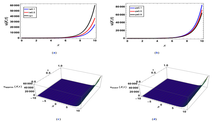
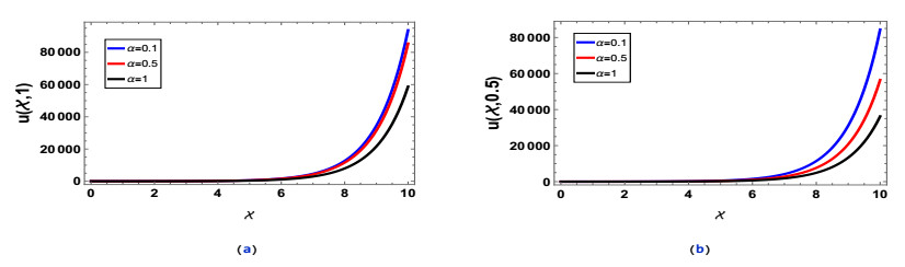
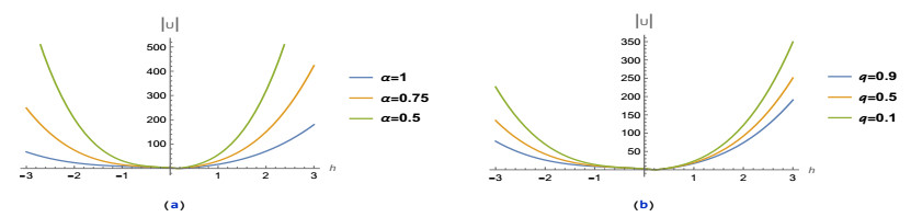
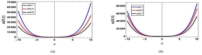
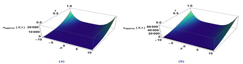
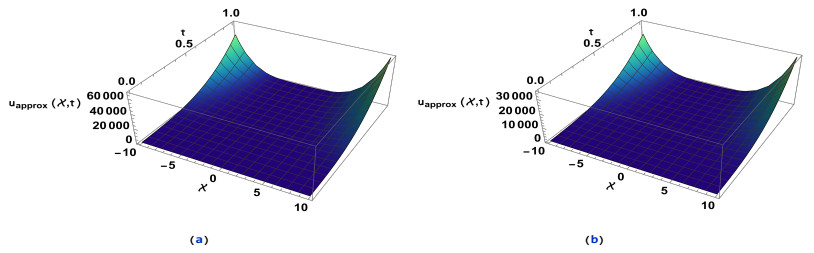
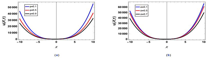
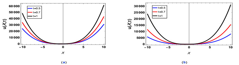
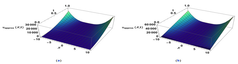
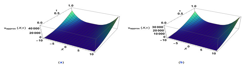
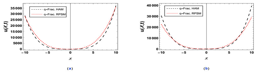
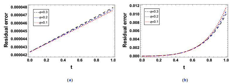
1.   Introduction

In recent decades, there has been a significant rise in research and developments within the field of fractional calculus. Numerous studies have explored the historical evolution of fractional calculus and its applications in various engineering aspects ^[1,2], physics ^[3], financial ^[4], and even in implementing natural phenomenon ^[5]. All of these applications are modeled by fractional differential equations that have been solved using analytical and numerical techniques ^[6,7,8,9]. Recently, considerable focus has been directed towards $\mathit{q}$-calculus and $\mathit{q}$-fractional differential equations ($\mathit{q}$-FDEs) by mathematicians and engineers, because it bridges physics and mathematics. The inception of $\mathit{q}$-calculus, alternatively referred to as quantum calculus, traces back to 1908 with Jackson's contributions ^[10]. Building upon $\mathit{q}$-calculus, $\mathit{q}$-differential equations were formulated to depict specific physical phenomena observed in the dynamics of quantum systems, discrete dynamic systems, and related areas. As the $\mathit{q}$-calculus theory has advanced, several associated ideas have been presented and scrutinized. These include the $\mathit{q}$-Laplace transform, the $\mathit{q}$-Mittag Leffler function, the $\mathit{q}$-Gamma, and $\mathit{q}$-Beta functions ^[11], $\mathit{q}$-integral transforms, the $\mathit{q}$-Taylor series ^[12,13,14], and similar subjects, see ^[15]. As of now, investigations into $\mathit{q}$-fractional calculus is in its initial phases and has been compared with traditional fractional calculus. $\mathit{q}$-differential equations have found applications in modeling both linear and nonlinear problems, thus playing a crucial role across various domains in engineering and science. While many studies have provided research outcomes concerning the uniqueness of the solutions and also the existence of various types of $\mathit{q}$-FDEs, there is a limited number of studies that have focused on the analytical solution of these problems ^[16,17]. Some studies have addressed solving $\mathit{q}$-differential equations without merging fractional calculus into them, thereby using semi-analytical methods, such as the $\mathit{q}$-differential transform method ^[18,19,20], the homotopy analysis method ^[21], the variation iteration method ^[22,23], and the $\mathit{q}$-separation of variable method ^[24]. Until now, the study and investigation of fractional $\mathit{q}$-calculus is still in its nascent phase, specially when solving $\mathit{q}$-FDEs using analytical and semi-analytical techniques. Currently the only methods that have been are the fractional $\mathit{q}$-Laplace transform ^[13,14], the fractional $\mathit{q}$-Laplace transform in time scale ^[25], and the fractional $\mathit{q}$-reduced differential transform ^[26,27]. Since there are some semi-analytical methods that provide a high accuracy in the results and are used to solve fractional order differential equations, our aim is to apply these methods to the $\mathit{q}$-differential equations due to the importance of $\mathit{q}$-calculus in quantum theory, which connects physics with its applications and mathematics. Recently, B. Madhavi and others published a paper that focused on solving $\mathit{q}$-FDEs using the Homotopy Analysis Method (HAM); however, they applied the method for two simple ordinary differential equations ^[28].

In this study, we aim to investigate and solve linear and nonlinear $\mathit{q}$-FPDEs using the HAM and the Residual Power Series Method (RPSM). Both the RPSM and the HAM provide solutions in the form of a series that approximates the exact solution of a problem. One of the key advantages of the HAM is its flexibility, as it introduces an auxiliary parameter (often referred to as $\hbar$) that allows the user to control and adjust the convergence region of the series solution, see ^[29]. This capability enables the HAM to offer a better control over the accuracy and convergence of the solution, especially in problems where traditional methods struggle with a slow convergence. Additionally, the HAM is highly versatile and can be applied to a wide range of linear and nonlinear problems, thus making it suitable for more complex systems. However, the method may suffer from a slow convergence when dealing with strongly nonlinear equations, thus potentially requiring a higher computational effort to achieve accurate results. On the other hand, the RPSM transforms the differential equation into a series of algebraic equations, which can significantly simplify the solution process, particularly for nonlinear problems. It is relatively straightforward to implement compared to other semi-analytical methods; and can handle a wide range of nonlinearities without the need for linearization or perturbation. Moreover, the RPSM tends to work well even in the presence of strong nonlinearity, thereby providing accurate approximations. Another advantage of the RPSM is that it provides closed-form solutions for each term in the series, allowing for a clear interpretation of the solution's behavior. Nevertheless, the accuracy of the solution depends on the number of terms retained in the series, meaning that a higher accuracy often demands a larger number of terms, which can increase the computational effort. It is worth mentioning that this is the first time these methods have been used to solve $\mathit{q}$-FDEs.

This study is structured as follows: In Section 2, we introduce the fundamental definitions and notations of fractional $\mathit{q}$-calculus; Section 3 is concerned with the implementation of the RPSM; and the HAM and how to use these methods to solve $\mathit{q}$-FPDEs; in Section 4, numerical examples are given to illustrate the effectiveness of the suggested methods; representations of the obtained solutions in 2D and 3D are showcased in Section 5; and Section 6 presents the conclusion of this study.

2.   Basic notations of $\mathit{q}$-calculus

Within this part, we introduce the condensed basics of the fundamental definitions and characteristics of $\mathcal{q}$-calculus, along with fractional $\mathit{q}$-derivatives and integrals. For a more comprehensive understanding, additional specifics can be found in ^[30,31].

Definition 2.1. ^[14]. Consider a real-valued function, denoted by $\varOmega(\mathfrak{t})$, defined on a set $\mathscr{T}_\mathit{q} = \{\mathit{q}^\vartheta:\vartheta \in \mathcal{Z}\} \cup \{0\}$, where $0 < \mathit{q} < 1$, which is a geometric set, and $\mathcal{Z}$ is the set of integer numbers. Then, the $\mathit{q}-derivative$ of $\varOmega(\mathfrak{t})$ is defined as follows:

From the Definition 2.1, it is evident that the $\mathit{q}$-derivative differs from the traditional derivative, which can be regarded as a discrete analogue of the traditional derivative.

It is worth mentioning that $\lim_{\mathit{q}\rightarrow 1} D_\mathit{q}\varOmega(\mathfrak{t}) = \frac{d\varOmega(\mathfrak{t})}{d\mathfrak{t}}$. For a higher order $\mathit{q}$-derivative,

For any functions $\mathcal{U}(\mathfrak{t})$ and $\mathcal{V}(\mathfrak{t})$, which are considered functions with real values, the following properties are valid:

Definition 2.2. ^[26]. For a higher order $\mathit{q}$-derivative, and any two functions $\mathcal{U}(\mathcal{X})$ and $\mathcal{V}(\mathcal{X})$,

where

and

Definition 2.3. ^[26]. The $\mathit{q}$-analogue of $(\mathcal{X}-\mathfrak{a})_\mathit{q}^\vartheta$ is a polynomial:

Now, let's focus and shed light on the definitions specific to fractional $\mathit{q}$-calculus.

Definition 2.4. ^[14]. For ${\beta} \neq -1, -2, ...$, where ${\beta}$ is the fractional order $\mathit{q}$-derivative, the Riemann-Liouville (RL) fractional $\mathit{q}$-integral is characterized by the following definition:

where $\Gamma_\mathit{q}({\beta})$ is the $\mathit{q}$-analogue Gamma function, which is defined as follows:

where

From the definition of $\Gamma_\mathit{q}({\beta})$, one can easily verify that:

Definition 2.5. ^[14]. Suppose $\varOmega(\mathfrak{t})$ is a positive real-valued function, for $\vartheta = [{\beta}]$. In that case, the fractional $\mathit{q}$-derivative in sense of Caputo of order ${\beta}$ is given by the following:

where $[{\beta}]$ denotes the smallest integer greater than or equal to ${\beta}$. At ${\beta} > 0$,

Definition 2.6. ^[26,32]. Assume that $\varOmega(\mathfrak{t})$ is a real-valued function $\in \mathsf{R}^+$; for $\vartheta = [{\beta}]$, ${\beta}\in \mathsf{R}$; then, the RL fractional $\mathit{q}$-derivative of order ${\beta}$ is as follows:

At ${\beta} > 0$,

For a real valued function $f(\mathfrak{t})$, where $\alpha, {\beta}$ are the fractional parameters, the following properties are established, and their proofs are presented in ^[13,14,33]:

3.   Implementation of HAM and RPSM

In this part, we will explore how the semi-analytical approaches (HAM and RPSM) are adapted to be applicable to the $\mathit{q}$-FPDEs in the following form:

where $0 < \mathit{q} < 1$ and the fractional order derivative $0 < \alpha \leq 1$, thereby utilizing the initial approximation:

3.1.   Preliminaries of $\mathit{q}$-fractional HAM

The HAM was initially introduced and implemented by Liao ^[34,35]; moreover, it has been adapted to address extremely nonlinear and complex FDEs and a system of FDEs, see ^[36,37]. In this work, the HAM will be adapted to be applicable to the $\mathit{q}$-FPDEs.

Equation (3.1) can be reformulated as follows:

and is conditioned by the following:

where $\mathscr{N}$ is called the nonlinear operator. We can formulate the $zero-order \, \mathit{q}$-deformation equation as follows:

In Eq (3.3), we consider the unknown function $\mathcal{Q}(\mathcal{X}, \mathfrak{t}, \mathfrak{p})$, which involves an embedding parameter $\mathfrak{p}$ within the range $[0, 1]$, a non-zero auxiliary parameter $\mathsf{h}$, and an auxiliary function $\mathsf{H}(\mathcal{X}, \mathfrak{t})$. Clearly, if $\mathfrak{p} = 0$, then $\mathcal{Q}(\mathcal{X}, \mathfrak{t}, 0) = \varXi_0(\mathcal{X}, \mathfrak{t})$, and for $\mathfrak{p} = 1$, $\mathcal{Q}(\mathcal{X}, \mathfrak{t}, 1) = \varXi(\mathcal{X}, \mathfrak{t})$. As $\mathfrak{p}$ ascends between $0$ and $1$, the solution undergoes variation between the beginning condition $\varXi_0(\mathcal{X}, \mathfrak{t})$ and the estimated solution $\varXi(\mathcal{X}, \mathfrak{t})$.

$\mathcal{Q}$ can be expressed as a Taylor series expansion in relation to the parameter $\mathfrak{p}$,

in which

The solution in the series form may be expressed in the following format:

To prove the previous steps, consider the subsequent theorem:

Theorem 3.1. For the series (3.4) that presents the homotopy series, it can be formulated as follows:

where, the following relations are true:

i. $\frac{1}{[\mathbf{m}]_\mathit{q}!} \frac{\partial^\mathbf{m}_\mathit{q}\mathcal{Q} }{\partial_\mathit{q}\mathfrak{p}^\mathbf{m}}|_{\mathfrak{p} = 0} = \varXi_\mathbf{m}(\mathcal{X}, \mathfrak{t})$,    ii. $\frac{1}{[\mathbf{m}]_\mathit{q}!} \frac{\partial^\mathbf{m}_\mathit{q}(\mathfrak{p}\mathcal{Q}) }{\partial_\mathit{q}\mathfrak{p}^\mathbf{m}}|_{\mathfrak{p} = 0} = \varXi_\mathbf{m-1}(\mathcal{X}, \mathfrak{t})$,

iii. $\frac{1}{[\mathbf{m}]_\mathit{q}!} \frac{\partial^\mathbf{m}_\mathit{q}(\mathfrak{p^2}\mathcal{Q}) }{\partial_\mathit{q}\mathfrak{p}^\mathbf{m}}|_{\mathfrak{p} = 0} = \varXi_\mathbf{m-2}(\mathcal{X}, \mathfrak{t})$, ... and so on.

Proof. By using the $\mathit{q}$-Taylor series presented in ^[12,33], the first relation $(i)$ is directly proven.

For $(ii)$, from Eq (3.8),

Hence, $\frac{\partial^\mathbf{m}_\mathit{q}(\mathfrak{p}\mathcal{Q}) }{\partial_\mathit{q}\mathfrak{p}^\mathbf{m}}$ exists when $\mathsf{j} = \mathbf{m-1}$, and $\frac{1}{[\mathbf{m}]_\mathit{q}!} \frac{\partial^\mathbf{m}_\mathit{q}(\mathfrak{p}\mathcal{Q}) }{\partial_\mathit{q}\mathfrak{p}^\mathbf{m}}|_{\mathfrak{p} = 0} = \varXi_\mathbf{m-1}(\mathcal{X}, \mathfrak{t})$.

In the same manner, we can prove $iii$. □

To find the higher terms $\varXi_\mathbf{m}(\mathcal{X}, \mathfrak{t})$, we will use the following vector:

To find the $\mathit{q}$-deformation equation of the $\mathbf{m}$-th order, we differentiate Eq (3.3) $\mathbf{m}$ times with respect to $\mathfrak{p}$; after that, we put $\mathfrak{p} = 0$, divide by $[\mathbf{m}]_\mathit{q}!$, and obtain the following:

in which

and

3.2.   Preliminaries of $\mathit{q}$-fractional RPSM

In this part, we modify the RPSM that has been implemented for fractional patial differential equations ^[38,39] to be applicable to the $\mathit{q}$-FPDEs. Follow the following steps to solve the $\mathit{q}$-FPDEs in the form of Eq (3.1).

Step 1. The solution can be expressed as a series of the $\mathit{q}$- fractional power series centered around $\mathfrak{t} = 0$, thereby adopting the following structure:

Step 2. Define the $\mathfrak{n}$th truncated series,

where $\mathsf{g}(\mathcal{X})$ is the initial condition $\varXi_0(\mathcal{X}, \mathfrak{t})$.

Step 3. Define the $\mathfrak{n}$th residual function,

Step 4. Substitute the $\mathfrak{n}$th series (3.13) into the $\mathfrak{n}$th function (3.14).

Step 5. Incorporate the $\mathsf{i}$th series of $\varXi_\mathsf{i}(\mathcal{X}, \mathfrak{t})$ into Eq (3.14). Utilize the $\mathit{q}$-derivative in the fractional form $D_{\mathfrak{t}, \mathit{q}}^{(\mathfrak{n}-1)\alpha}$ at $\mathfrak{t} = 0$ to ascertain the required coefficients $\mathsf{g}_{\mathsf{i}}(\mathcal{X})$ for $\mathsf{i} = 1, 2, 3, ..., \mathfrak{n}$.

Step 6. By solving the set of $\mathit{q}$ algebraic equations,

we obtain the coefficients $\mathsf{g}_{\mathsf{i}}(\mathcal{X})$ for the assumed power series (3.12).

3.3.   Convergence analysis

Since the two proposed solution methods yield the approximate solution in a series form, this section focuses on studying the convergence of the solution. Consider the truncated power series that represents the solution of the following form:

with exact solution $\varXi(\mathcal{X}, \mathfrak{t})$. Assume the general form of the equation under study in the following form:

Theorem 3.2. Let $\mathbb{F}$ represent an operator mapping from $\mathbb{H}$ to $\mathbb{H}$ (where $\mathbb{H}$ denotes the Hilbert space), and suppose $\varXi$ denotes the exact solution of Eq (3.17). Then, the approximate solution (3.16) converges to $\varXi$ if there exists a constant $\varepsilon$, with $0 < \varepsilon \leq 1$, such that $\parallel \mathsf{g}_{\kappa+1}(\mathcal{X}, \mathfrak{t}) \parallel \leq \varepsilon \parallel \mathsf{g}_{\kappa}(\mathcal{X}, \mathfrak{t}) \parallel$ holds for all $\kappa \in \mathbb{N} \cup \{0\}$.

Proof. We want to prove that $\mathsf{g}_ \mathsf{J} |_{\mathsf{J} = 0}^\infty$ is a convergent Cauchy sequence,

For $\mathsf{J}, \text{ı}\in N, \, \mathsf{J} > \text{ı}$,

Hence, $\mathsf{g}_ \mathsf{J}|_{\mathsf{J} = 0}^\infty$ is a convergent Cauchy sequence in $\mathbb{H}$. □

4.   Applications

In this part, we will present the solution of two equations. Additionally, one linear ($\mathit{q}$-fractional diffusion equation); and the other nonlinear (nonlinear $\mathit{q}$-fractional PDE), we will solve each of them using both methods: The $\mathit{q}$-fractional HAM and the $\mathit{q}$-fractional RPSM.

4.1.   $\mathit{q}$-fractional diffusion equation

Assume the equation in the following form:

which is subject to the following:

Note that ^[18],

Using the $\mathit{q}$-fractional HAM: Following the steps introduced in Section (3.1), the solution is expressed in the following form:

where

By setting $\mathbf{m} = 1$ and implying the properties presented in Eqs (2.9)–(2.12),

Setting $\mathbf{m} = 2$,

We can continue in the same sequence, hence,

When putting $\alpha = 1$, it is worth noting that, the solution in approximation form is as follows:

From Definition 2.4,

From Definition 2.2, $[\vartheta]_\mathit{q} = \mathit{q}^{\vartheta-1}+...+\mathit{q}+1$, hence,

Therefore, (4.8) is simplified as follows:

which is the same solution derived in ^[21]. Additionally, when putting $\mathsf{h} = -1$, in Eq (4.9), the solution becomes the exact solution as presented in ^[18,21]:

The exact solution is $\mathbf{u}(\mathcal{X}, \mathfrak{t}) = e_\mathit{q}^\mathcal{X} e_\mathit{q}^\mathfrak{t}$.

Table 1 represents the absolute error between the exact solutions and the approximate solutions (Five terms) for $\alpha = 1$ and $\mathfrak{t} = 0.1$ for different values of $\mathsf{h}$ and $\mathit{q}$. From the results, we note that, the approximate solution becomes the exact solution at $\mathsf{h} = -1$ and $\mathit{q}\rightarrow1$.

Now, we will solve the same Eq (4.1) using the $\mathit{q}$-fractional RPSM.

Using the $\mathit{q}$-fractional RPSM: Following the steps introduced in Section (3.2), let the solution be formatted as follows:

where $\mathsf{g}_0(\mathcal{X})$ represents the starting condition $\mathbf{u}(\mathcal{X}, 0) = e_\mathit{q}^\mathcal{X}$. Our aim is to evaluate $\mathsf{g}_1(\mathcal{X}), \mathsf{g}_2(\mathcal{X}), ...$ The $\mathfrak{n}$th residual function is as follows:

For the first residual,

where

By substituting Eq (4.14) into Eq (4.13),

By applying the condition $Res_{\mathbf{u}_{\mathit{q}, 1}}(\mathcal{X}, \mathfrak{t}) = 0$ at $\mathfrak{t} = 0$, we acquire the value of $\mathsf{g}_1(\mathcal{X})$ as follows:

The second residual is as follows:

where

By substituting (4.18) into Eq (4.17),

By applying the condition $D_{\mathfrak{t}, \mathit{q}}^{\alpha} Res_{\mathbf{u}_{\mathit{q}, 2}}(\mathcal{X}, \mathfrak{t}) = 0$ at $\mathfrak{t} = 0$, we acquire the following value of $\mathsf{g}_2(\mathcal{X})$:

We can continue to find higher terms in the series solution including $\mathsf{g}_3(\mathcal{X}), \mathsf{g}_4(\mathcal{X}), ...$. The approximate series solution will be obtained when substituting the values of $\mathsf{g}_0(\mathcal{X}), \mathsf{g}_1(\mathcal{X}), \mathsf{g}_2(\mathcal{X}), ...$ in Eq (4.11) as follows:

From Eq (4.21), it is evident that the solution obtained through the $\mathit{q}$-fractional RPSM matches with the solution obtained through the $\mathit{q}$-fractional HAM, which confirms the validity of this method to the $\mathit{q}$-FPDEs.

At $\alpha = 1$, the approximate solution becomes the following:

which is also the solution obtained in ^[18,21].

4.2.   Nonlinear $\mathit{q}$-fractional PDE

Consider the nonlinear $\mathit{q}$-FPDE in the following form:

under the initial guess

Using the $\mathit{q}$-fractional HAM: The approximate truncated series is expressed as follows:

where; the $\mathbf{m}$-th order $\mathit{q}$-deformation equation is as follows:

For $\mathbf{m} = 1$, we obtain the first iteration:

For $\mathbf{m} = 2$,

By setting $\mathbf{m} = 3$, we find $\mathbf{u}_3(\mathcal{X}, \mathfrak{t})$, and so forth; consequently, the result solution will be as follows:

Table 2 represents the residual error of the nonlinear $\mathit{q}$-FPDE (4.23) using the $\mathit{q}$-fractional HAM when only expanding 3 terms. The results are obtained at $\alpha = 1$ and $\mathsf{h} = -1$ for different values of $\mathit{q}$ and different steps of time.

Table 3 provides the residual error of the nonlinear $\mathit{q}$-FPDE (4.23) using the$\mathit{q}$-fractional HAM at $\mathsf{h} = -1$ for $\mathit{q}\rightarrow1$ at different values of $\alpha$ and different steps of time. The results reflect the accuracy of the obtained solutions, although the results we obtained are derived by expanding only three approximate terms.

Using the $\mathit{q}$-fractional RPSM: The solution can be represented as follows:

where $\mathsf{g}_0(\mathcal{X})$ is the starting condition $\mathbf{u}(\mathcal{X}, 0) = 1+3\mathcal{X}$. The $\mathfrak{n}$th residual function is as follows:

At $\mathfrak{n} = 1$, we obtain the first residual:

where

By substituting (4.32) into Eq (4.31), we obtain the following,

By applying the condition $Res_{\mathbf{u}_{\mathit{q}, 1}}(\mathcal{X}, \mathfrak{t}) = 0$ at $\mathfrak{t} = 0$, we acquire the following value of $\mathsf{g}_1(\mathcal{X})$:

For the second residual,

where

By substituting from Eq (4.36) into Eq (4.35), we obtain the following:

This is due to the following:

By applying the condition $D_{\mathfrak{t}, \mathit{q}}^{\alpha} Res_{\mathbf{u}_\mathit{q}, 2}(\mathcal{X}, \mathfrak{t}) = 0$ at $\mathfrak{t} = 0$ in Eq (4.37), we acquire $\mathsf{g}_2(\mathcal{X})$:

If we continue on the same sequence, then we can find higher terms $\mathsf{g}_3(\mathcal{X}), \mathsf{g}_4(\mathcal{X}), ...$, then substitute it into Eq (4.29). The approximate series solution will be as follows:

It is worth mentioning that, if we substitute by $\alpha = 1$ into the series solution (4.39), then we obtain the following:

which is the same solution obtained when solving this problem using the reduced $\mathit{q}$-differential transform method presented in ^[20]. All the results we obtained were obtained with the aid of the Mathematica 13.2 software.

Table 4 represents the residual error for solving the nonlinear $\mathit{q}$-FPDE (4.23) using the $\mathit{q}$-fractional RPSM at $\mathfrak{t} = 0.1$ for different values of $\alpha$ when $\mathit{q}\longrightarrow1$ and different values of $\mathit{q}$ at $\alpha = 1$.

5.   Visual representations

Visual representations provide a graphical environment that enriches the understanding of the data and outcomes. They provide an immediate and intuitive understanding of the relationships and patterns present in the data, thus facilitating a more accessible comprehension for both researchers and readers to appreciate the importance of the results.

In this study, we present two- and three-dimensional representations for the obtained solutions from solving linear and nonlinear problems using two methods: The $\mathit{q}$-fractional HAM and the $\mathit{q}$-fractional RPSM. Figure 1 depicts the solution to the diffusion Eq (4.1). Figure 1(a) and (b) clarify the two-dimensional solution when $\alpha = 1$ at various time instances $\mathfrak{t} = 1$ and $\mathit{q}$, respectively. Figure 1(c) represents the 3D representation of the obtained solution at $\alpha = 1$ and $\mathit{q\rightarrow1}$. Figure 1(d) represents the exact solution at $\alpha = 1$ and $\mathit{q\rightarrow1}$. From the 3D representation, we notice a significant match between the solution obtained from using the two proposed methods and the exact solution, thus indicating the efficiency of the methods in solving the problem. Figure 2 offers the 2D visualization of the solution of the diffusion equation for various fractional order derivative values $\alpha$ at $\mathit{q\rightarrow1}$ across different time intervals.

Additionally, we present a nonlinear problem (4.23) and clarify the solution using the two proposed methods: The $\mathit{q}$-fractional HAM and the $\mathit{q}$-fractional RPSM. When solving the problem using the $\mathit{q}$-fractional HAM, the solution depends on an optimal parameter $\mathsf{h}$. Figure 3 clarifies the $\mathsf{h}$-curves in which the convergence region is defined as the area parallel to the $x$-axis. Figure 3(a) illustrates the curves for $\mathsf{h}$ at various $\alpha$ values. Figure 3(b) illustrates the curves for $\mathsf{h}$ at different $\mathit{q}$ values; from the figure, we note that the region is approximately within $[-0.6, 0.5]$. Figure 4 represents the 2D visualization of the nonlinear problem (4.23) when solved by the $\mathit{q}$-fractional HAM at time $\mathfrak{t} = 1$ and $\mathsf{h} = 0.4$. In Figure 4(a), we offer the solution at various $\mathit{q}$ values when $\alpha = 1$. In Figure 4(b), the solution is presented for $\mathit{q\rightarrow1}$ with different $\alpha$ values. Figure 5(a) and (b) show the 3D visualizations of the $\mathit{q}$-fractional HAM at $\mathfrak{t} = 1, \mathsf{h} = 0.4$, and $\mathit{q\rightarrow1}$ for $\alpha = 1$ and $\alpha = 0.5$, respectively. Figures 6(a) and 5(b) show the 3D profiles of the $\mathit{q}$-fractional HAM at $\mathfrak{t} = 1, \mathsf{h} = 0.4$, and $\alpha = 1$ for $\mathit{q = 0.1}$ and $\mathit{q = 0.7}$, respectively. Figure 7 depicts the 2D profile of the solution for the nonlinear $\mathit{q}$-fractional PDE using the $\mathit{q}$-fractional RPSM at fixed time $\mathfrak{t} = 1$. Figure 7(a) shows the approximated solution at $\alpha = 1$ for several values of $\mathit{q}$. Figure 7(b) offers the solution at $\mathit{q\rightarrow1}$ for different sets of $\alpha$. Figures 8(a) and (b) clarify the solutions of the $\mathit{q}$-fractional PDE at fixed $\mathit{q\rightarrow1}$ at several stages of time for $\alpha = 0.5$ and $\alpha = 1$, respectively. Figure 9(a) and (b) clarify the 3D profiles at a fixed time and $\mathit{q}$ for $\alpha = 1$ and $\alpha = 0.5$. Figure 10(a) and (b) represent the 3D profile at fixed time and $\alpha$ for $\mathit{q} = 0.1$ and $\mathit{q} = 0.7$, respectively. Because the nonlinear problem presented in Eq (4.23) has no known exact solution, Figure 11 clarifies a contrast between the solutions approximated using the $\mathit{q}$-fractional HAM and the $\mathit{q}$-fractional RPSM at $\mathit{q = 0.7}$. Figure 11(a) at $\mathsf{h} = 0.4$ and $\mathfrak{t} = 1$, and Figure 11(b) at $\mathsf{h} = 0.5$ and $\mathfrak{t} = 0.9$. The curves are very close together, which indicates the efficiency of the two methods. To demonstrate the efficiency of the methods and the accuracy of the solutions we obtained, especially for the nonlinear $\mathit{q}$-fractional PDE represented in Eq (4.23), we plotted residual error curves since the exact solution of the equation is unknown. Figure 12 represents the residual error using the $\mathit{q}$-fractional HAM at $\alpha = 1.$ Figure 12(a) represents the error at $\mathsf{h} = -0.01$, and Figure 12(b) represents the error at $\mathsf{h} = -1$. It is noted that the accuracy of the solution is better at the value of $\mathsf{h} = -0.01$, which is consistent with the $\mathsf{h}$-curves. Figure 13 represents the residual error using the $\mathit{q}$-fractional HAM at different values of $\alpha$ and $\mathit{q} \longrightarrow 1.$ Figure 13(a) represents the error at $\mathsf{h} = -0.01$, and Figure 13(b) represents the error at $\mathsf{h} = -1.$ Figure 14 clarifies the residual error using the $\mathit{q}$-fractional RPSM. Figure 14(a) represents the error at $\alpha = 1$ and distinct $\mathit{q}$ values, and Figure 14(b) represents the error at several values of $\alpha$ for $\mathit{q}\longrightarrow1$.

6.   Conclusions

This paper introduced a novel methodology to tackle $\mathit{q}$-fractional partial differential equations by integrating the RPSM and the HAM. The utilization of these semi-analytical methods was extended to derive approximate solutions for both linear and nonlinear $\mathit{q}$-FPDEs. The outcomes of this study affirm the accuracy of the obtained solutions. The significance of $\mathit{q}$-FPDEs in $\mathit{q}$-calculus, particularly their relevance in engineering applications and quantum mechanics, has motivated the exploration of innovative approaches for their resolution. We presented the obtained solutions in 2D and 3D graphs to show the significance of the parameters on each other and on the solutions. To demonstrate the precision and effectiveness of the proposed methods, we compared the solutions we obtained with other published papers at the same parameters.

For future directions, we will enhance and generalize the proposed methods to handle the $\mathit{q}$-fractional PDEs which have applications in quantum calculus in higher dimensions, such as, the $\mathit{q}$-fractional Navier-Stokes equations in 3-dim, the $\mathit{q}$-fractional Korteweg-de'Vries (KdV) equation, the $\mathit{q}$-fractional Schrödinger equation, and others. The primary challenge lies in handling the increased complexity that arises from multiple spatial dimensions, which increases the number of coupled differential equations. However, both the RPSM and the HAM can be systematically extended to tackle such problems. Additionally, we will try to explore specific applications that arise in quantum mechanics. Moreover, we can also can use the time-scale approach with $\mathit{q}$-FPDEs to solve relevant challenges in the domains of physics and engineering.

Author contributions

The authors declare that the study was realized in collaboration with equal responsibility. All authors have read and approved the final version of the manuscript for publication.

Acknowledgment

The authors extend their appreciation to Taif University, Saudi Arabia, for supporting this work through project number (TU-DSPP-2024-73).

Funding

This research was funded by Taif University, Saudi Arabia, Project No. (TU-DSPP-2024-73).

Conflict of interest

There is no conflict of interest between the authors or anyone else regarding this manuscript.