A novel class of forward-backward explicit iterative algorithms using inertial techniques to solve variational inequality problems with quasi-monotone operators

Bancha Panyanak; Chainarong Khunpanuk; Nattawut Pholasa; Nuttapol Pakkaranang; Bancha Panyanak; Chainarong Khunpanuk; Nattawut Pholasa; Nuttapol Pakkaranang

doi:10.3934/math.2023489

AIMS Mathematics

2023, Volume 8, Issue 4: 9692-9715. doi: 10.3934/math.2023489

Previous Article Next Article

Research article

A novel class of forward-backward explicit iterative algorithms using inertial techniques to solve variational inequality problems with quasi-monotone operators

1.
Research Group in Mathematics and Applied Mathematics, Department of Mathematics, Faculty of Science, Chiang Mai University, Chiang Mai 50200, Thailand
2.
Data Science Research Center, Department of Mathematics, Faculty of Science, Chiang Mai University, Chiang Mai 50200, Thailand
3.
Mathematics and Computing Science Program, Faculty of Science and Technology, Phetchabun Rajabhat University, Phetchabun 67000, Thailand
4.
School of Science, University of Phayao, Phayao 56000, Thailand

Received: 13 November 2022 Revised: 02 February 2023 Accepted: 05 February 2023 Published: 21 February 2023
MSC : 47H05, 47H10, 47J20, 47J25, 65J15, 91B50

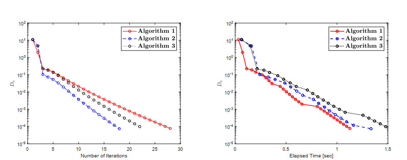
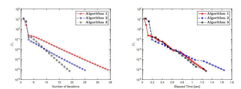
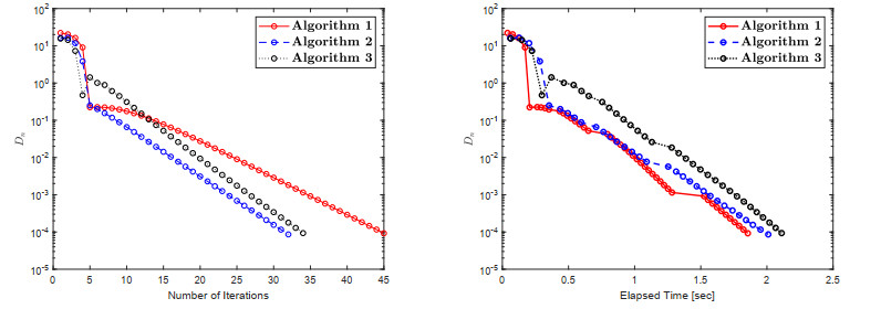
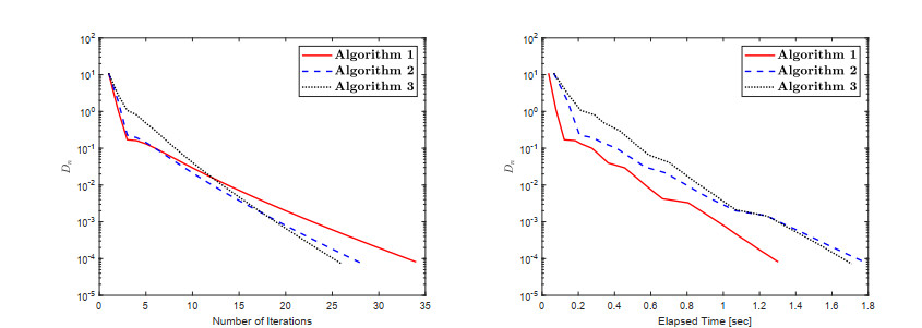
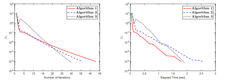
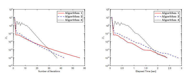
The theory of variational inequalities is an important tool in physics, engineering, finance, and optimization theory. The projection algorithm and its variants are useful tools for determining the approximate solution to the variational inequality problem. This paper introduces three distinct extragradient algorithms for dealing with variational inequality problems involving quasi-monotone and semistrictly quasi-monotone operators in infinite-dimensional real Hilbert spaces. This problem is a general mathematical model that incorporates a set of applied mathematical models as an example, such as equilibrium models, optimization problems, fixed point problems, saddle point problems, and Nash equilibrium point problems. The proposed algorithms employ both fixed and variable stepsize rules that are iteratively transformed based on previous iterations. These algorithms are based on the fact that no prior knowledge of the Lipschitz constant or any line-search framework is required. To demonstrate the convergence of the proposed algorithms, some simple conditions are used. Numerous experiments have been conducted to highlight the numerical capabilities of algorithms.
- variational inequalities,
- Tseng's extragradient method,
- inertial-type iterative scheme,
- quasi-monotone operator,
- Lipschitz continuous operators
Citation: Bancha Panyanak, Chainarong Khunpanuk, Nattawut Pholasa, Nuttapol Pakkaranang. A novel class of forward-backward explicit iterative algorithms using inertial techniques to solve variational inequality problems with quasi-monotone operators[J]. AIMS Mathematics, 2023, 8(4): 9692-9715. doi: 10.3934/math.2023489

Related Papers:

Abstract

The theory of variational inequalities is an important tool in physics, engineering, finance, and optimization theory. The projection algorithm and its variants are useful tools for determining the approximate solution to the variational inequality problem. This paper introduces three distinct extragradient algorithms for dealing with variational inequality problems involving quasi-monotone and semistrictly quasi-monotone operators in infinite-dimensional real Hilbert spaces. This problem is a general mathematical model that incorporates a set of applied mathematical models as an example, such as equilibrium models, optimization problems, fixed point problems, saddle point problems, and Nash equilibrium point problems. The proposed algorithms employ both fixed and variable stepsize rules that are iteratively transformed based on previous iterations. These algorithms are based on the fact that no prior knowledge of the Lipschitz constant or any line-search framework is required. To demonstrate the convergence of the proposed algorithms, some simple conditions are used. Numerous experiments have been conducted to highlight the numerical capabilities of algorithms.

References

[1]	A. Antipin, On a method for convex programs using a symmetrical modification of the lagrange function, Ekonomika i Matematicheskie Metody, 12 (1976), 1164–1173.
[2]	T. Bantaojai, N. Pakkaranang, H. ur Rehman, P. Kumam, W. Kumam, Convergence analysis of self-adaptive inertial extra-gradient method for solving a family of pseudomonotone equilibrium problems with application, Symmetry, 12 (2020), 1332. http://dx.doi.org/10.3390/sym12081332 doi: 10.3390/sym12081332
[3]	L. Ceng, A. Petrușel, X. Qin, J. Yao, A modified inertial subgradient extragradient method for solving pseudomonotone variational inequalities and common fixed point problems, Fixed Point Theory, 21 (2020), 93–108. http://dx.doi.org/10.24193/fpt-ro.2020.1.07 doi: 10.24193/fpt-ro.2020.1.07
[4]	L. Ceng, A. Petrușel, C. Wen, J. Yao, Inertial-like subgradient extragradient methods for variational inequalities and fixed points of asymptotically nonexpansive and strictly pseudocontractive mappings, Mathematics, 7 (2019), 860. http://dx.doi.org/10.3390/math7090860 doi: 10.3390/math7090860
[5]	L. Ceng, A. Petrușel, J. Yao, On mann viscosity subgradient extragradient algorithms for fixed point problems of finitely many strict pseudocontractions and variational inequalities, Mathematics, 7 (2019), 925. http://dx.doi.org/10.3390/math7100925 doi: 10.3390/math7100925
[6]	L. Ceng, M. Shang, Composite extragradient implicit rule for solving a hierarch variational inequality with constraints of variational inclusion and fixed point problems, J. Inequal. Appl., 2020 (2020), 33. http://dx.doi.org/10.1186/s13660-020-2306-1 doi: 10.1186/s13660-020-2306-1
[7]	L. Ceng, C. Wen, Y. Liou, J. Yao, A general class of differential hemivariational inequalities systems in reflexive banach spaces, Mathematics, 9 (2021), 3173. http://dx.doi.org/10.3390/math9243173 doi: 10.3390/math9243173
[8]	Y. Censor, A. Gibali, S. Reich, The subgradient extragradient method for solving variational inequalities in hilbert space, J. Optim. Theory Appl., 148 (2011), 318–335. http://dx.doi.org/10.1007/s10957-010-9757-3 doi: 10.1007/s10957-010-9757-3
[9]	Y. Censor, A. Gibali, S. Reich, Strong convergence of subgradient extragradient methods for the variational inequality problem in hilbert space, Optim. Method. Softw., 26 (2011), 827–845. http://dx.doi.org/10.1080/10556788.2010.551536 doi: 10.1080/10556788.2010.551536
[10]	Y. Censor, A. Gibali, S. Reich, Extensions of korpelevich extragradient method for the variational inequality problem in euclidean space, Optimization, 61 (2012), 1119–1132. http://dx.doi.org/10.1080/02331934.2010.539689 doi: 10.1080/02331934.2010.539689
[11]	S. Chang, Salahuddin, L. Wang, M. Liu, On the weak convergence for solving semistrictly quasi-monotone variational inequality problems, J. Inequal. Appl., 2019 (2019), 74. http://dx.doi.org/10.1186/s13660-019-2032-8 doi: 10.1186/s13660-019-2032-8
[12]	C. Elliott, Variational and quasivariational inequalities applications to free-boundary problems, SIAM Review, 29 (1987), 314–315. http://dx.doi.org/10.1137/1029059
[13]	G. Grillo, G. Stampacchia, Formes bilinéaires coercitives sur les ensembles convexes, Académie des Sciences de Paris, 258 (1964), 4413–4416.
[14]	N. Hadjisavvas, S. Schaible, On strong pseudomonotonicity and (semi)strict quasimonotonicity, J. Optim. Theory Appl., 79 (1993), 139–155. http://dx.doi.org/10.1007/BF00941891 doi: 10.1007/BF00941891
[15]	L. He, Y. Cui, L. Ceng, T. Zhao, D. Wang, H. Hu, Strong convergence for monotone bilevel equilibria with constraints of variational inequalities and fixed points using subgradient extragradient implicit rule, J. Inequal. Appl., 2021 (2021), 146. http://dx.doi.org/10.1186/s13660-021-02683-y doi: 10.1186/s13660-021-02683-y
[16]	A. Iusem, B. Svaiter, A variant of korpelevich's method for variational inequalities with a new search strategy, Optimization, 42 (1997), 309–321. http://dx.doi.org/10.1080/02331939708844365 doi: 10.1080/02331939708844365
[17]	G. Kassay, J. Kolumbán, Z. Páles, On nash stationary points, Publ. Math. Debrecen, 54 (1999), 267–279. http://dx.doi.org/10.5486/pmd.1999.1902 doi: 10.5486/pmd.1999.1902
[18]	G. Kassay, J. Kolumbán, Z. Páles, Factorization of minty and stampacchia variational inequality systems, Eur. J. Oper. Res., 143 (2002), 377–389. http://dx.doi.org/10.1016/S0377-2217(02)00290-4 doi: 10.1016/S0377-2217(02)00290-4
[19]	D. Kinderlehrer, G. Stampacchia, An introduction to variational inequalities and their applications, New York: Society for Industrial and Applied Mathematics, 2000. http://dx.doi.org/10.1137/1.9780898719451
[20]	I. Konnov, Equilibrium models and variational inequalities, New York: Elsevier, 2007.
[21]	G. Korpelevich, The extragradient method for finding saddle points and other problems, Matecon, 12 (1976), 747–756.
[22]	H. Liu, J. Yang, Weak convergence of iterative methods for solving quasimonotone variational inequalities, Comput. Optim. Appl., 77 (2020), 491–508. http://dx.doi.org/10.1007/s10589-020-00217-8 doi: 10.1007/s10589-020-00217-8
[23]	L. Liu, Ishikawa and mann iterative process with errors for nonlinear strongly accretive mappings in banach spaces, J. Math. Anal. Appl., 194 (1995), 114–125. http://dx.doi.org/10.1006/jmaa.1995.1289 doi: 10.1006/jmaa.1995.1289
[24]	L. Liu, S. Cho, J. Yao, Convergence analysis of an inertial tseng's extragradient algorithm for solving pseudomonotone variational inequalities and applications, J. Nonlinear Var. Anal., 5 (2021), 627–644. http://dx.doi.org/10.23952/jnva.5.2021.4.09 doi: 10.23952/jnva.5.2021.4.09
[25]	P. Maingé, Strong convergence of projected subgradient methods for nonsmooth and nonstrictly convex minimization, Set-Valued Anal., 16 (2008), 899–912. http://dx.doi.org/10.1007/s11228-008-0102-z doi: 10.1007/s11228-008-0102-z
[26]	A. Moudafi, Viscosity approximation methods for fixed-points problems, J. Math. Anal. Appl., 241 (2000), 46–55. http://dx.doi.org/10.1006/jmaa.1999.6615 doi: 10.1006/jmaa.1999.6615
[27]	A. Nagurney, Network economics: a variational inequality approach, New York: Springer, 1999. http://dx.doi.org/10.1007/978-1-4757-3005-0
[28]	M. Noor, Some iterative methods for nonconvex variational inequalities, Comput. Math. Model., 21 (2010), 97–108. http://dx.doi.org/10.1007/s10598-010-9057-7 doi: 10.1007/s10598-010-9057-7
[29]	P. Peeyada, W. Cholamjiak, D. Yambangwai, A hybrid inertial parallel subgradient extragradient-line algorithm for variational inequalities with an application to image recovery, J. Nonlinear Funct. Anal., 2022 (2022), 9. http://dx.doi.org/ 10.23952/jnfa.2022.9 doi: 10.23952/jnfa.2022.9
[30]	S. Regmi, Optimized iterative methods with applications in diverse disciplines, New York: Nova Science Publishers, 2020.
[31]	Salahuddin, The extragradient method for quasi-monotone variational inequalities, Optimization, 71 (2022), 2519–2528. http://dx.doi.org/10.1080/02331934.2020.1860979
[32]	B. Tan, S. Cho, J. Yao, Accelerated inertial subgradient extragradient algorithms with non-monotonic step sizes for equilibrium problems and fixed point problems, J. Nonlinear Var. Anal., 6 (2022), 89–122. http://dx.doi.org/10.23952/jnva.6.2022.1.06 doi: 10.23952/jnva.6.2022.1.06
[33]	B. Tan, S. Li, Revisiting projection and contraction algorithms for solving variational inequalities and applications, Applied Set-Valued Analysis and Optimization, 4 (2022), 167–183. http://dx.doi.org/10.23952/asvao.4.2022.2.03 doi: 10.23952/asvao.4.2022.2.03
[34]	B. Tan, X. Qin, S. Cho, Revisiting subgradient extragradient methods for solving variational inequalities, Numer. Algor., 90 (2022), 1593–1615. http://dx.doi.org/10.1007/s11075-021-01243-1 doi: 10.1007/s11075-021-01243-1
[35]	B. Tan, X. Qin, J. Yao, Strong convergence of inertial projection and contraction methods for pseudomonotone variational inequalities with applications to optimal control problems, J. Glob. Optim., 82 (2022), 523–557. http://dx.doi.org/10.1007/s10898-021-01095-y doi: 10.1007/s10898-021-01095-y
[36]	B. Tan, X. Qin, J. Yao, Strong convergence of self-adaptive inertial algorithms for solving split variational inclusion problems with applications, J. Sci. Comput., 87 (2021), 20. http://dx.doi.org/10.1007/s10915-021-01428-9 doi: 10.1007/s10915-021-01428-9
[37]	P. Tseng, A modified forward-backward splitting method for maximal monotone mappings, SIAM J. Control Optim., 38 (2000), 431–446. http://dx.doi.org/10.1137/S0363012998338806
[38]	H. ur Rehman, M. Özdemir, I. Karahan, N. Wairojjana, The Tseng's extragradient method for semistrictly quasimonotone variational inequalities, J. Appl. Numer. Optim., 4 (2022), 203–214.
[39]	H. ur Rehman, A. Gibali, P. Kumam, K. Sitthithakerngkiet, Two new extragradient methods for solving equilibrium problems, RACSAM, 115 (2021), 75. http://dx.doi.org/10.1007/s13398-021-01017-3 doi: 10.1007/s13398-021-01017-3
[40]	H. ur Rehman, P. Kumam, Y. Cho, P. Yordsorn, Weak convergence of explicit extragradient algorithms for solving equilibirum problems, J. Inequal. Appl., 2019 (2019), 282. http://dx.doi.org/10.1186/s13660-019-2233-1 doi: 10.1186/s13660-019-2233-1
[41]	H. ur Rehman, P. Kumam, A. Gibali, W. Kumam, Convergence analysis of a general inertial projection-type method for solving pseudomonotone equilibrium problems with applications, J. Inequal. Appl., 2021 (2021), 63. http://dx.doi.org/10.1186/s13660-021-02591-1 doi: 10.1186/s13660-021-02591-1
[42]	H. ur Rehman, P. Kumam, Y. Cho, Y. Suleiman, W. Kumam, Modified popov's explicit iterative algorithms for solving pseudomonotone equilibrium problems, Optim. Method. Soft., 36 (2021), 82–113. http://dx.doi.org/10.1080/10556788.2020.1734805 doi: 10.1080/10556788.2020.1734805
[43]	H. ur Rehman, W. Kumam, P. Kumam, M. Shutaywi, A new weak convergence non-monotonic self-adaptive iterative scheme for solving equilibrium problems, AIMS Mathematics, 6 (2021), 5612–5638. http://dx.doi.org/10.3934/math.2021332 doi: 10.3934/math.2021332
[44]	H. ur Rehman, N. Pakkaranang, A. Hussain, N. Wairojjana, A modified extra-gradient method for a family of strongly pseudomonotone equilibrium problems in real Hilbert spaces, J. Math. Comput. Sci., 22 (2021), 38–48. http://dx.doi.org/10.22436/jmcs.022.01.04 doi: 10.22436/jmcs.022.01.04
[45]	N. Wairojjana, H. ur Rehman, I. Argyros, N. Pakkaranang, An accelerated extragradient method for solving pseudomonotone equilibrium problems with applications, Axioms, 9 (2020), 99. http://dx.doi.org/10.3390/axioms9030099 doi: 10.3390/axioms9030099
[46]	Y. Wang, T. Xu, J. Yao, B. Jiang, Self-adaptive method and inertial modification for solving the split feasibility problem and fixed-point problem of quasi-nonexpansive mapping, Mathematics, 10 (2022), 1612. http://dx.doi.org/10.3390/math10091612 doi: 10.3390/math10091612
[47]	J. Yang, H. Liu, A modified projected gradient method for monotone variational inequalities, J. Optim. Theory Appl., 179 (2018), 197–211. http://dx.doi.org/10.1007/s10957-018-1351-0 doi: 10.1007/s10957-018-1351-0
[48]	J. Yang, H. Liu, Z. Liu, Modified subgradient extragradient algorithms for solving monotone variational inequalities, Optimization, 67 (2018), 2247–2258. http://dx.doi.org/10.1080/02331934.2018.1523404 doi: 10.1080/02331934.2018.1523404
[49]	L. Zhang, C. Fang, S. Chen, An inertial subgradient-type method for solving single-valued variational inequalities and fixed point problems, Numer. Algor., 79 (2018), 941–956. http://dx.doi.org/10.1007/s11075-017-0468-9 doi: 10.1007/s11075-017-0468-9

Reader Comments

Your name:*

Email:*
© 2023 the Author(s), licensee AIMS Press. This is an open access article distributed under the terms of the Creative Commons Attribution License (http://creativecommons.org/licenses/by/4.0)