Surface family pair with Bertrand pair as mutual geodesic curves in Euclidean 3-space $ \mathbb{E}^{3} $

Areej A. Almoneef; Rashad A. Abdel-Baky; Areej A. Almoneef; Rashad A. Abdel-Baky

doi:10.3934/math.20231047

AIMS Mathematics

2023, Volume 8, Issue 9: 20546-20560. doi: 10.3934/math.20231047

Previous Article Next Article

Research article

Surface family pair with Bertrand pair as mutual geodesic curves in Euclidean 3-space $ \mathbb{E}^{3} $

Areej A. Almoneef ^{1
,
,},
Rashad A. Abdel-Baky ²

1.
Department of Mathematical Sciences, College of Science, Princess Nourah bint Abdulrahman University, P.O. Box 84428, Riyadh 11671, Saudi Arabia
2.
Department of Mathematics, Faculty of Science, University of Assiut 71516, Egypt

Received: 14 May 2023 Revised: 17 June 2023 Accepted: 20 June 2023 Published: 26 June 2023
MSC : 53A04, 53A05, 53A17

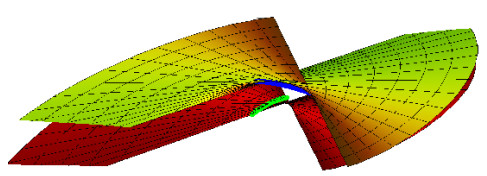
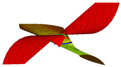
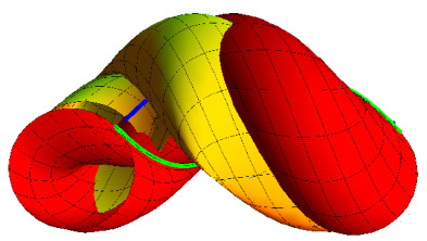
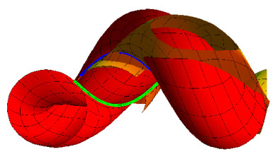
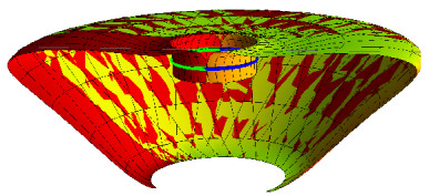
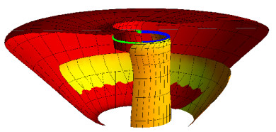
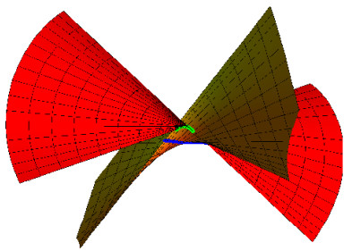
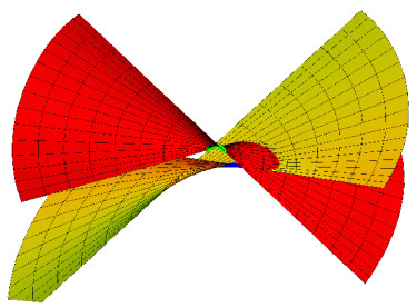
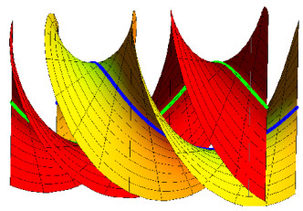
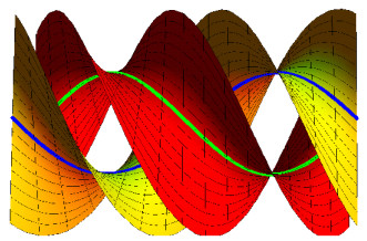
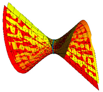
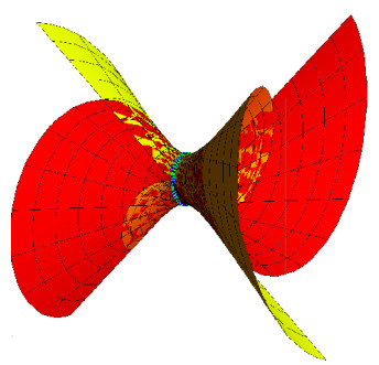
The main interest of this work is to construct surface family pair with the symmetry of Bertrand pair in Euclidean 3-space $ \mathbb{E}^{3} $. Then, by employing the Serret-Frenet frame, we conclude the sufficient and necessary conditions of surface family pair interpolating Bertrand pair as mutual geodesic curves. Moreover, the conclusion to ruled surface family pair is also obtained. Meanwhile, this work is demonstrated through several examples.
- geodesic curve,
- Bertrand mate,
- ruled surface
Citation: Areej A. Almoneef, Rashad A. Abdel-Baky. Surface family pair with Bertrand pair as mutual geodesic curves in Euclidean 3-space $ \mathbb{E}^{3} $[J]. AIMS Mathematics, 2023, 8(9): 20546-20560. doi: 10.3934/math.20231047

Related Papers:

Abstract

The main interest of this work is to construct surface family pair with the symmetry of Bertrand pair in Euclidean 3-space $ \mathbb{E}^{3} $. Then, by employing the Serret-Frenet frame, we conclude the sufficient and necessary conditions of surface family pair interpolating Bertrand pair as mutual geodesic curves. Moreover, the conclusion to ruled surface family pair is also obtained. Meanwhile, this work is demonstrated through several examples.

References

[1]	M. Do Carmo, Differential geometry of curves and surfaces, Englewood Cliffs: Prentice-Hall, 1976.
[2]	M. Spivak, A comprehensive introduction to differential geometry, 2 Eds., Houston: Publish or Perish, 1979.
[3]	R. Brond, D. Jeulin, P. Gateau, J. Jarrin, G. Serpe, Estimation of the transport properties of polymer composites by geodesic propagation, J. Microsc., 176 (1994), 167–177. http://dx.doi.org/10.1111/j.1365-2818.1994.tb03511.x doi: 10.1111/j.1365-2818.1994.tb03511.x
[4]	S. Bryson, Virtual spacetime: an environment for the visualization of curved spacetimes via geodesic flows, Proceedings of Visualization, 1992,291–298. http://dx.doi.org/10.1109/VISUAL.1992.235196 doi: 10.1109/VISUAL.1992.235196
[5]	R. Haw, An application of geodesic curves to sail design, Comput. Graph. Forum, 4 (1985), 137–139. http://dx.doi.org/10.1111/j.1467-8659.1985.tb00203.x doi: 10.1111/j.1467-8659.1985.tb00203.x
[6]	R. Haw, F. Munchmeyer, Geodesic curves on patched polynomial surfaces, Comput. Graph. Forum, 2 (1983), 225–232. http://dx.doi.org/10.1111/j.1467-8659.1983.tb00151.x doi: 10.1111/j.1467-8659.1983.tb00151.x
[7]	P. Agarwal, S. Har-Peled, M. Sharir, K. Varadarajan, Approximating shortest paths on a convex polytope in three dimensions, J. ACM, 44 (1997), 567–584. http://dx.doi.org/10.1145/263867.263869 doi: 10.1145/263867.263869
[8]	R. Goldenberg, R. Kimmel, E. Rivlin, M. Rudzsky, Fast geodesic active contours, IEEE Trans. Image Process., 10 (2001), 1467–1475. http://dx.doi.org/10.1109/83.951533 doi: 10.1109/83.951533
[9]	S. Har-Peled, Approximate shortest-path and geodesic diameter on convex polytopes in three dimensions, Discrete Comput. Geom., 21 (1999), 217–231. http://dx.doi.org/10.1007/PL00009417 doi: 10.1007/PL00009417
[10]	M. Novotni, R. Klein, Gomputing geodesic distances on triangular meshes, Journal of WSCG, 10 (2002), 341–347.
[11]	G. Wang, K. Tang, C. Tai, Parametric representation of a surface pencil with a common spatial geodesic, Comput. Aided Design, 36 (2004), 447–459. http://dx.doi.org/10.1016/S0010-4485(03)00117-9 doi: 10.1016/S0010-4485(03)00117-9
[12]	H. Zhao, G. Wang, A new method for designing a developable surface utilizing the surface pencil through a given curve, Prog. Nat. Sci., 18 (2008), 105–110. http://dx.doi.org/10.1016/j.pnsc.2007.09.001 doi: 10.1016/j.pnsc.2007.09.001
[13]	C. Li, R. Wang, C. Zhu, Design and G1 connection of developable surfaces through Bézier geodesics, Appl. Math. Comput., 218 (2011), 3199–3208. http://dx.doi.org/10.1016/j.amc.2011.08.057 doi: 10.1016/j.amc.2011.08.057
[14]	E. Kasap, F. Talay Akyildiz, K. Orbay, A generalization of surfaces family with common spatial geodesic, Appl. Math. Comput., 201 (2008), 781–789. http://dx.doi.org/10.1016/j.amc.2008.01.016 doi: 10.1016/j.amc.2008.01.016
[15]	C. Li, R. Wang, C. Zhu, Parametric representation of a surface pencil with a common line of curvature, Comput. Aided Design, 43 (2011), 1110–1117. http://dx.doi.org/10.1016/j.cad.2011.05.001 doi: 10.1016/j.cad.2011.05.001
[16]	C. Li, R. Wang, C. Zhu, An approach for designing a developable surface through a given line of curvature, Comput. Aided Design, 45 (2013), 621–627. http://dx.doi.org/10.1016/j.cad.2012.11.001 doi: 10.1016/j.cad.2012.11.001
[17]	E. Bayram, F. Guler, E. Kasap, Parametric representation of a surface pencil with a common asymptotic curve, Comput. Aided Design, 44 (2012), 637–643. http://dx.doi.org/10.1016/j.cad.2012.02.007 doi: 10.1016/j.cad.2012.02.007
[18]	Y. Liu, G. Wang, Designing developable surface pencil through given curve as its common asymptotic curve (Chinese), Journal of Zhejiang University (Engineering Science), 47 (2013), 1246–1252. http://dx.doi.org/10.3785/j.issn.1008-973X.2013.07.017 doi: 10.3785/j.issn.1008-973X.2013.07.017
[19]	G. Atalay, E. Kasap, Surfaces family with common Smarandache geodesic curve, J. Sci. Arts, 17 (2017), 651–664.
[20]	G. Atalay, E. Kasap, Surfaces family with common Smarandache geodesic curve according to Bishop frame in Euclidean space, Mathematical Sciences and Applications E-Notes, 4 (2016), 164–174. http://dx.doi.org/10.36753/mathenot.421425 doi: 10.36753/mathenot.421425
[21]	E. Bayram, M. Bilici, Surface family with a common involute asymptotic curve, Int. J. Geom. Methods M., 13 (2016) 1650062. http://dx.doi.org/10.1142/S0219887816500626. doi: 10.1142/S0219887816500626
[22]	F. Güler, E. Bayram, E. Kasap, Offset surface pencil with a common asymptotic curve, Int. J. Geom. Methods M., 15 (2018), 1850195. http://dx.doi.org/10.1142/S0219887818501955 doi: 10.1142/S0219887818501955
[23]	G. Atalay, Surfaces family with a common Mannheim asymptotic curve, Journal of Applied Mathematics and Computation, 2 (2018), 143–154. http://dx.doi.org/10.26855/jamc.2018.04.004 doi: 10.26855/jamc.2018.04.004
[24]	G. Atalay, Surfaces family with a common Mannheim geodesic curve, Journal of Applied Mathematics and Computation, 2 (2018), 155–165. http://dx.doi.org/10.26855/jamc.2018.04.005 doi: 10.26855/jamc.2018.04.005
[25]	R. Abdel-Baky, N. Alluhaib, Surfaces family with a common geodesic curve in Euclidean 3-Space $\mathbb{E}^{3}$, International Journal of Mathematical Analysis, 13 (2019), 433–447. http://dx.doi.org/10.12988/ijma.2019.9846 doi: 10.12988/ijma.2019.9846
[26]	J. Watson, F. Crick, Molecular structures of nucleic acids, Nature, 171 (1953), 737–738. http://dx.doi.org/10.1038/171737a0 doi: 10.1038/171737a0
[27]	A. Jain, G. Wang, K. Vasquez, DNA triple helices: biological consequences and the therapeutic potential, Biochemie, 90 (2008), 1117–1130. http://dx.doi.org/10.1016/j.biochi.2008.02.011 doi: 10.1016/j.biochi.2008.02.011
[28]	L. Jäntschi, The Eigenproblem translated for alignment of molecules, Symmetry, 11 (2019), 1027. http://dx.doi.org/10.3390/sym11081027 doi: 10.3390/sym11081027
[29]	L. Jäntschi, S. Bolboaca, Study of geometrical shaping of linear chained polymers stabilized as helixes, Stud. UBB-Chem., 61 (2016), 123–136.
[30]	S. Papaioannou, D. Kiritsis, An application of Bertrand curves and surface to CAD/CAM, Comput. Aided Design, 17 (1985), 348–352. http://dx.doi.org/10.1016/0010-4485(85)90025-9 doi: 10.1016/0010-4485(85)90025-9
[31]	B. Ravani, T. Ku, Bertrand offsets of ruled and developable surfaces, Comput. Aided Design, 23 (1991), 145–152. http://dx.doi.org/10.1016/0010-4485(91)90005-H doi: 10.1016/0010-4485(91)90005-H

Reader Comments

Your name:*

Email:*
© 2023 the Author(s), licensee AIMS Press. This is an open access article distributed under the terms of the Creative Commons Attribution License (http://creativecommons.org/licenses/by/4.0)