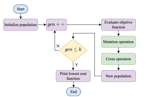
The optimization of fractional-order (FO) chaotic systems is challenging when simulating a considerable number of cases for long times, where the primary problem is verifying if the given parameter values will generate chaotic behavior. In this manner, we introduce a methodology for detecting chaotic behavior in FO systems through the analysis of Poincaré maps. The optimization process is performed applying differential evolution (DE) and accelerated particle swarm optimization (APSO) algorithms for maximizing the Kaplan-Yorke dimension ($ D_{KY} $) of two case studies: a 3D and a 4D FO chaotic systems with hidden attractors. These FO chaotic systems are solved applying the Grünwald-Letnikov method, and the Numba just-in-time (jit) compiler is used to improve the optimization process's time execution in Python programming language. The optimization results show that the proposed method efficiently optimizes FO chaotic systems with hidden attractors while saving execution time.
Citation: Daniel Clemente-López, Esteban Tlelo-Cuautle, Luis-Gerardo de la Fraga, José de Jesús Rangel-Magdaleno, Jesus Manuel Munoz-Pacheco. Poincaré maps for detecting chaos in fractional-order systems with hidden attractors for its Kaplan-Yorke dimension optimization[J]. AIMS Mathematics, 2022, 7(4): 5871-5894. doi: 10.3934/math.2022326
The optimization of fractional-order (FO) chaotic systems is challenging when simulating a considerable number of cases for long times, where the primary problem is verifying if the given parameter values will generate chaotic behavior. In this manner, we introduce a methodology for detecting chaotic behavior in FO systems through the analysis of Poincaré maps. The optimization process is performed applying differential evolution (DE) and accelerated particle swarm optimization (APSO) algorithms for maximizing the Kaplan-Yorke dimension ($ D_{KY} $) of two case studies: a 3D and a 4D FO chaotic systems with hidden attractors. These FO chaotic systems are solved applying the Grünwald-Letnikov method, and the Numba just-in-time (jit) compiler is used to improve the optimization process's time execution in Python programming language. The optimization results show that the proposed method efficiently optimizes FO chaotic systems with hidden attractors while saving execution time.

| [1] | Y. Bolotin, A. Tur, V. Yanovsky, Chaos: Concepts, control and constructive use, Springer, 2009. |
| [2] |
B. Dubey, Sajan, A. Kumar, Stability switching and chaos in a multiple delayed prey-predator model with fear effect and anti-predator behavior, Math. Comput. Simulat., 188 (2021), 164–192. https://doi.org/10.1016/j.matcom.2021.03.037 doi: 10.1016/j.matcom.2021.03.037

|
| [3] | J. K. Zink, K. Batygin, F. C. Adams, The great inequality and the dynamical disintegration of the outer solar system, Astron. J., 160 (2020), 232. |
| [4] | M. Sajid, Recent developments on chaos in mechanical systems, Int. J. Theor. Appl. Res. Mech. Eng., 2 (2013), 121–124. |
| [5] | B. A. Idowu, S. Vaidyanathan, A. Sambas, O. I. Olusola, O. S. Onma, A new chaotic finance system: Its analysis, control, synchronization and circuit design, In: Nonlinear dynamical systems with self-excited and hidden attractors, Springer, 2018,271–295. https://doi.org/10.1007/978-3-319-71243-7_12 |
| [6] |
B Wang, S. M. Zhong, X. C. Dong, On the novel chaotic secure communication scheme design, Commun. Nonlinear Sci. Numer. Simul., 39 (2016), 108–117. https://doi.org/10.1016/j.cnsns.2016.02.035 doi: 10.1016/j.cnsns.2016.02.035
|
| [7] |
D. Arroyo, F. Hernandez, A. B. Orúe, Cryptanalysis of a classical chaos-based cryptosystem with some quantum cryptography features, Int. J. Bifurcat. Chaos, 27 (2017), 1750004. https://doi.org/10.1142/S0218127417500043 doi: 10.1142/S0218127417500043
|
| [8] |
X. Zang, S. Iqbal, Y. Zhu, X. Liu, J. Zhao, Applications of chaotic dynamics in robotics, Int. J. Adv. Robotic Syst., 13 (2016), 60. https://doi.org/10.5772/62796 doi: 10.5772/62796
|
| [9] |
K. Tian, C. Grebogi, H. P. Ren, Chaos generation with impulse control: Application to non-chaotic systems and circuit design, IEEE T. Circuits Syst. I, 68 (2021), 3012–3022. https://doi.org/10.1109/TCSI.2021.3075550 doi: 10.1109/TCSI.2021.3075550
|
| [10] |
V. E. Tarasov, Generalized memory: Fractional calculus approach, Fractal Fract., 2 (2018), 23. https://doi.org/10.3390/fractalfract2040023 doi: 10.3390/fractalfract2040023
|
| [11] |
K. M. Owolabi, A. Atangana, J. F. Gómez-Aguilar, Fractional adams-bashforth scheme with the liouville-caputo derivative and application to chaotic systems, Discrete Cont. Dyn. Syst.-S, 14 (2021), 2455–2469. https://doi.org/10.3934/dcdss.2021060 doi: 10.3934/dcdss.2021060
|
| [12] |
M. Ahmad, U. Shamsi, I. R. Khan, An enhanced image encryption algorithm using fractional chaotic systems, Procedia Comput. Sci., 57 (2015), 852–859. https://doi.org/10.1016/j.procs.2015.07.494 doi: 10.1016/j.procs.2015.07.494
|
| [13] |
M. Bettayeb, U. M. Al-Saggaf, S. Djennoune, Single channel secure communication scheme based on synchronization of fractional-order chaotic Chua's systems, T. I. Meas. Control, 40 (2018), 3651–3664. https://doi.org/10.1177/0142331217729425 doi: 10.1177/0142331217729425
|
| [14] |
H. Natiq, M. R. M. Said, M. R. K. Ariffin, S. He, L. Rondoni, S. Banerjee, Self-excited and hidden attractors in a novel chaotic system with complicated multistability, Eur. Phys. J. Plus, 133 (2018), 1–12. https://doi.org/10.1140/epjp/i2018-12360-y doi: 10.1140/epjp/i2018-12360-y
|
| [15] |
G. A. Leonov, N. V. Kuznetsov, Hidden attractors in dynamical systems. From hidden oscillations in hilbert-kolmogorov, aizerman, and kalman problems to hidden chaotic attractor in chua circuits, Int. J. Bifurcat. Chaos, 23 (2013), 1330002. https://doi.org/10.1142/S0218127413300024 doi: 10.1142/S0218127413300024
|
| [16] |
P. R. Sharma, M. D. Shrimali, A. Prasad, N. V. Kuznetsov, G. A. Leonov, Control of multistability in hidden attractors, Eur. Phys. J. Spec. Top., 224 (2015), 1485–1491. https://doi.org/10.1140/epjst/e2015-02474-y doi: 10.1140/epjst/e2015-02474-y
|
| [17] |
A. K. Farhan, R. S. Ali, H. Natiq, N. M. G. Al-Saidi, A new s-box generation algorithm based on multistability behavior of a plasma perturbation model, IEEE Access, 7 (2019), 124914–124924. https://doi.org/10.1109/ACCESS.2019.2938513 doi: 10.1109/ACCESS.2019.2938513
|
| [18] |
F. Yu, Z. Zhang, L. Liu, H. Shen, Y. Huang, C. Shi, et al., Secure communication scheme based on a new 5D multistable four-wing memristive hyperchaotic system with disturbance inputs, Complexity, 2020 (2020), 5859273. https://doi.org/10.1155/2020/5859273 doi: 10.1155/2020/5859273
|
| [19] |
J. M. Munoz-Pacheco, E. Zambrano-Serrano, C. Volos, S. Jafari, J. Kengne, K. Rajagopal, A new fractional-order chaotic system with different families of hidden and self-excited attractors, Entropy, 20 (2018), 564. https://doi.org/10.3390/e20080564 doi: 10.3390/e20080564
|
| [20] |
N. Debbouche, S. Momani, A. Ouannas, M. T. Shatnawi, G. Grassi, Z. Dibi, et al., Generating multidirectional variable hidden attractors via newly commensurate and incommensurate non-equilibrium fractional-order chaotic systems, Entropy, 23 (2021), 261. https://doi.org/10.3390/e23030261 doi: 10.3390/e23030261
|
| [21] |
D. A. Yousri, A. M. AbdelAty, L. A. Said, A. S. Elwakil, B. Maundy, A. G. Radwan, Parameter identification of fractional-order chaotic systems using different meta-heuristic optimization algorithms, Nonlinear Dynam., 95 (2019), 2491–2542. https://doi.org/10.1007/s11071-018-4703-2 doi: 10.1007/s11071-018-4703-2
|
| [22] |
A. Silva-Juárez, E. Tlelo-Cuautle, L. G. de la Fraga, R. Li, Optimization of the kaplan-yorke dimension in fractional-order chaotic oscillators by metaheuristics, Appl. Math. Comput., 394 (2021), 125831. https://doi.org/10.1016/j.amc.2020.125831 doi: 10.1016/j.amc.2020.125831
|
| [23] |
J. C. Nunez-Perez, V. A. Adeyemi, Y. Sandoval-Ibarra, F. J. Perez-Pinal, E. Tlelo-Cuautle, Maximizing the chaotic behavior of fractional order chen system by evolutionary algorithms, Mathematics, 9 (2021), 1194. https://doi.org/10.3390/math9111194 doi: 10.3390/math9111194
|
| [24] |
S. Jafari, J. C. Sprott, F. Nazarimehr, Recent new examples of hidden attractors, Eur. Phys. J. Spec. Top., 224 (2015), 1469–1476. https://doi.org/10.1140/epjst/e2015-02472-1 doi: 10.1140/epjst/e2015-02472-1
|
| [25] |
W. S. Sayed, A. G. Radwan, Self-reproducing hidden attractors in fractional-order chaotic systems using affine transformations, IEEE Open J. Circuits Syst., 1 (2020), 243–254. https://doi.org/10.1109/OJCAS.2020.3030756 doi: 10.1109/OJCAS.2020.3030756
|
| [26] |
M. F. Danca, P. Bourke, N. Kuznetsov, Graphical structure of attraction basins of hidden chaotic attractors: The rabinovich-fabrikant system, Int. J. Bifurcat. Chaos, 29 (2019), 1930001. https://doi.org/10.1142/S0218127419300015 doi: 10.1142/S0218127419300015
|
| [27] | C. W. Kulp, B. J. Niskala, Characterization of time series data, 2017. |
| [28] |
S. Zamen, E. Dehghan-Niri, Observation and diagnosis of chaos in nonlinear acoustic waves using phase-space domain, J. Sound Vib., 463 (2019), 114959. https://doi.org/10.1016/j.jsv.2019.114959 doi: 10.1016/j.jsv.2019.114959
|
| [29] |
M. S. Abdelouahab, N. E. Hamri, The grünwald-letnikov fractional-order derivative with fixed memory length, Mediterr. J. Math., 13 (2016), 557–572. https://doi.org/10.1007/s00009-015-0525-3 doi: 10.1007/s00009-015-0525-3
|
| [30] | A. Carpinteri, F. Mainardi, Fractals and fractional calculus in continuum mechanics, Vol. 378, Springer, 2014. |
| [31] |
K. M. Owolabi, B. Karaagac, Chaotic and spatiotemporal oscillations in fractional reaction-diffusion system, Chaos Solitons Fract., 141 (2020), 110302. https://doi.org/10.1016/j.chaos.2020.110302 doi: 10.1016/j.chaos.2020.110302
|
| [32] |
L. F. Ávalos-Ruiz, J. F. Gomez-Aguilar, A. Atangana, K. M. Owolabi, On the dynamics of fractional maps with power-law, exponential decay and Mittag-Leffler memory, Chaos, Solitons Fract., 127 (2019), 364–388. https://doi.org/10.1016/j.chaos.2019.07.010 doi: 10.1016/j.chaos.2019.07.010
|
| [33] |
K. M. Owolabi, J. F. Gómez-Aguilar, G. Fernández-Anaya, J. E. Lavín-Delgado, E. Hernández-Castillo, Modelling of chaotic processes with caputo fractional order derivative, Entropy, 22 (2020), 1027. https://doi.org/10.3390/e22091027 doi: 10.3390/e22091027
|
| [34] |
K. M. Owolabi, Computational techniques for highly oscillatory and chaotic wave problems with fractional-order operator, Eur. Phys. J. Plus, 135 (2020), 1–23. https://doi.org/10.1140/epjp/s13360-020-00873-z doi: 10.1140/epjp/s13360-020-00873-z
|
| [35] |
K. M. Owolabi, Robust synchronization of chaotic fractional-order systems with shifted chebyshev spectral collocation method, J. Appl. Anal., 27, 2021. https://doi.org/10.1515/jaa-2021-2053 doi: 10.1515/jaa-2021-2053
|
| [36] |
C. Li, C. Tao, On the fractional adams method, Comput. Math. Appl., 58 (2009), 1573–1588. https://doi.org/10.1016/j.camwa.2009.07.050 doi: 10.1016/j.camwa.2009.07.050
|
| [37] |
R. Scherer, S. L. Kalla, Y. Tang, J. Huang, The Grünwald-Letnikov method for fractional differential equations, Comput. Math. Appl., 62 (2011), 902–917. https://doi.org/10.1016/j.camwa.2011.03.054 doi: 10.1016/j.camwa.2011.03.054
|
| [38] | I. Petráš, Fractional-order nonlinear systems: Modeling, analysis and simulation, Springer Science & Business Media, 2011. |
| [39] |
S. Pooseh, R. Almeida, D. F. M. Torres, Discrete direct methods in the fractional calculus of variations, Comput. Math. Appl., 66 (2013), 668–676. https://doi.org/10.1016/j.camwa.2013.01.045 doi: 10.1016/j.camwa.2013.01.045
|
| [40] | P. A. Cook, Nonlinear dynamical systems, 2 Eds., Prentice Hall International (UK) Ltd., GBR, 1994. |
| [41] |
M. H. Arshad, M. Kassas, A. E. Hussein, M. A. Abido, A simple technique for studying chaos using jerk equation with discrete time sine map, Appl. Sci., 11 (2021), 437. https://doi.org/10.3390/app11010437 doi: 10.3390/app11010437
|
| [42] |
L. Chen, W. Pan, J. A. T. Machado, A. M. Lopes, R. Wu, Y. He, Design of fractional-order hyper-chaotic multi-scroll systems based on hysteresis series, Eur. Phys. J. Spec. Top., 226 (2017), 3775–3789. https://doi.org/10.1140/epjst/e2018-00012-8 doi: 10.1140/epjst/e2018-00012-8
|
| [43] |
M. Z. De la Hoz, L. Acho, Y. Vidal, A modified chua chaotic oscillator and its application to secure communications, Appl. Math. Comput., 247 (2014), 712–722. https://doi.org/10.1016/j.amc.2014.09.031 doi: 10.1016/j.amc.2014.09.031
|
| [44] |
J. Theiler, Estimating fractal dimension, JOSA A, 7 (1990), 1055–1073. https://doi.org/10.1364/JOSAA.7.001055 doi: 10.1364/JOSAA.7.001055
|
| [45] |
S. Haykin, S. Puthusserypady, Chaotic dynamics of sea clutter, Chaos: Interdisc. J. Nonlinear Sci., 7 (1997), 777–802. https://doi.org/10.1063/1.166275 doi: 10.1063/1.166275
|
| [46] |
K. E. Chlouverakis, Color maps of the kaplan–yorke dimension in optically driven lasers: Maximizing the dimension and almost-hamiltonian chaos, Int. J. Bifurcat. Chaos, 15 (2005), 3011–3021. https://doi.org/10.1142/S0218127405013848 doi: 10.1142/S0218127405013848
|
| [47] |
C. R. Suribabu, Differential evolution algorithm for optimal design of water distribution networks, J. Hydroinform., 12 (2010), 66–82. https://doi.org/10.2166/hydro.2010.014 doi: 10.2166/hydro.2010.014
|
| [48] | G. G. Wang, A. H. Gandomi, X. S. Yang, A. H. Alavi, A novel improved accelerated particle swarm optimization algorithm for global numerical optimization, Eng. Comput., 31 (2014). |
| [49] |
M. S. Tavazoei, M. Haeri, A proof for non existence of periodic solutions in time invariant fractional order systems, Automatica, 45 (2009), 1886–1890. https://doi.org/10.1016/j.automatica.2009.04.001 doi: 10.1016/j.automatica.2009.04.001
|
| [50] |
E. Kaslik, S. Sivasundaram, Non-existence of periodic solutions in fractional-order dynamical systems and a remarkable difference between integer and fractional-order derivatives of periodic functions, Nonlinear Anal.: Real World Appl., 13 (2012), 1489–1497. https://doi.org/10.1016/j.nonrwa.2011.11.013 doi: 10.1016/j.nonrwa.2011.11.013
|
| [51] |
C. Li, J. C. Sprott, Coexisting hidden attractors in a 4-d simplified lorenz system, Int. J. Bifurcat. Chaos, 24 (2014), 1450034. https://doi.org/10.1142/S0218127414500345 doi: 10.1142/S0218127414500345
|
| [52] |
M. Wang, X. Liao, Y. Deng, Z. Li, Y. Su, Y. Zeng, Dynamics, synchronization and circuit implementation of a simple fractional-order chaotic system with hidden attractors, Chaos, Solitons Fract., 130 (2020), 109406. https://doi.org/10.1016/j.chaos.2019.109406 doi: 10.1016/j.chaos.2019.109406
|
| [53] | Numba: A high performance python compiler, 2021. Available from: http://numba.pydata.org/. |
| [54] | N. Watkinson, P. Tai, A. Nicolau, A. Veidenbaum, Numbasummarizer: A python library for simplified vectorization reports, In: 2020 IEEE International Parallel and Distributed Processing Symposium Workshops (IPDPSW), IEEE, 2020, 1–7. https://doi.org/10.1109/IPDPSW50202.2020.00058 |


Figures(12) / Tables(6)

Daniel Clemente-López, Esteban Tlelo-Cuautle, Luis-Gerardo de la Fraga, José de Jesús Rangel-Magdaleno, Jesus Manuel Munoz-Pacheco. Poincaré maps for detecting chaos in fractional-order systems with hidden attractors for its Kaplan-Yorke dimension optimization[J]. AIMS Mathematics, 2022, 7(4): 5871-5894. doi: 10.3934/math.2022326


 DownLoad: