An iteration process for a general class of contractive-like operators: Convergence, stability and polynomiography

Ti-Ming Yu; Abdul Aziz Shahid; Khurram Shabbir; Nehad Ali Shah; Yong-Min Li; Ti-Ming Yu; Abdul Aziz Shahid; Khurram Shabbir; Nehad Ali Shah; Yong-Min Li

doi:10.3934/math.2021393

AIMS Mathematics

2021, Volume 6, Issue 7: 6699-6714. doi: 10.3934/math.2021393

Previous Article Next Article

Research article Special Issues

An iteration process for a general class of contractive-like operators: Convergence, stability and polynomiography

1.
School of Economic Information Engineering, Southwestern University of Finance and Economics, Chengdu 611130, China
2.
Department of Mathematics and Statistics, University of Lahore, Lahore 54000, Pakistan
3.
Department of Mathematics, GC University, Lahore 54000, Pakistan
4.
Department of Mechanical Engineering, Sejong University, Seoul 05006, Korea
5.
Department of Mathematics, Lahore Leads University, Lahore, Pakistan
6.
Department of Mathematics, Huzhou University, Huzhou 313000, China

Received: 26 December 2020 Accepted: 31 March 2021 Published: 19 April 2021
MSC : 34N05, 35A23

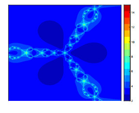
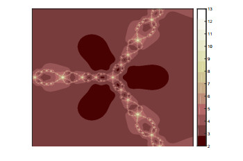
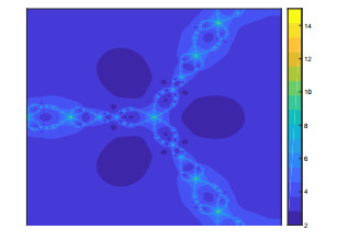
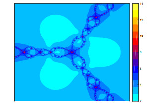
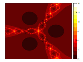
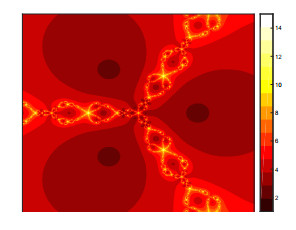
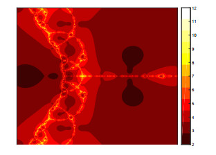
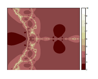
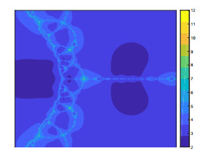
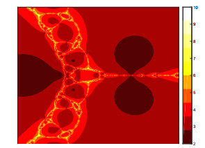
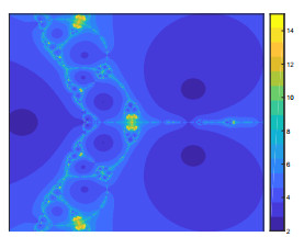
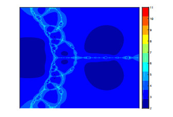
In this paper, we propose a three step iteration process and analyze the performance of the process for a contractive-like operators. It is observed that this iterative procedure is faster than several iterative methods in the existing literature. To support the claim, a numerical example is presented using Maple 13. Some images are generated by using this iteration method for complex cubic polynomials. We believe that our presented work enrich the polynomiography software.
- iterative schemes,
- image generation,
- contractive-like operators,
- convergence,
- polynomials
Citation: Ti-Ming Yu, Abdul Aziz Shahid, Khurram Shabbir, Nehad Ali Shah, Yong-Min Li. An iteration process for a general class of contractive-like operators: Convergence, stability and polynomiography[J]. AIMS Mathematics, 2021, 6(7): 6699-6714. doi: 10.3934/math.2021393

Related Papers:

Abstract

In this paper, we propose a three step iteration process and analyze the performance of the process for a contractive-like operators. It is observed that this iterative procedure is faster than several iterative methods in the existing literature. To support the claim, a numerical example is presented using Maple 13. Some images are generated by using this iteration method for complex cubic polynomials. We believe that our presented work enrich the polynomiography software.

References

[1]	W. R. Mann, Mean value methods in iteration, Proc. Am. Math. Soc., 4 (1953), 506–510. doi: 10.1090/S0002-9939-1953-0054846-3
[2]	S. Ishikawa, Fixed points by a new iteration method, Proc. Am. Math. Soc., 44 (1974), 147–150. doi: 10.1090/S0002-9939-1974-0336469-5
[3]	R. Agarwal, D. O. Regan, D. R. Sahu, Iterative construction of fixed points of nearly asymptotically nonexpansive mappings, J. Nonlinear Convex Anal., 8 (2007), 61.
[4]	M. A. Noor, New approximation schemes for general variational inequalities, J. Math. Anal. Appl., 251 (2000), 217–229. doi: 10.1006/jmaa.2000.7042
[5]	W. Phuengrattana, S. Suantai, On the rate of convergence of Mann, Ishikawa, Noor and SP-iterations for continuous functions on an arbitrary interval, J. Comput. Appl. Math., 235 (2011), 3006–3014. doi: 10.1016/j.cam.2010.12.022
[6]	R. Chugh, V. Kumar, S. Kumar, Strong convergence of a new three step iterative scheme in banach spaces, Am. J. Comput. Math., 2 (2012), 345. doi: 10.4236/ajcm.2012.24048
[7]	M. Abbas, T. Nazir, A new faster iteration process applied to constrained minimization and feasibility problems, Matematiqki Vesnik, 66 (2014), 223–234.
[8]	S. H. Khan, A Picard-Mann hybrid iterative process, Fixed Point Theory Appl., 2013 (2013), 1–10. doi: 10.1186/1687-1812-2013-1
[9]	F. Gürsoy, V. Karakaya, A Picard-S hybrid type iteration method for solving a differential equation with retarded argument, 2014. Available from: https://arXiv.org/abs/1403.2546.
[10]	N. Kadioglu, I. Yildirim, Approximating fixed points of nonexpansive mappings by a faster iteration process, 2014. Available from: https://arXiv.org/abs/1402.6530.
[11]	B. Rhoades, Some fixed point iteration procedures, Int. J. Math. Math.Sci., 14 (1991), 1–16. doi: 10.1155/S0161171291000017
[12]	V. Karakaya, F. Gürsoy, M. Ertürk, Comparison of the speed of convergence among various iterative schemes, 2014. Available from: https://arXiv.org/abs/1402.6080.
[13]	S. E. Mukiawa, The effect of time-varying delay damping on the stability of porous elastic system, Open J. Math. Sci., 5 (2021), 147–161.
[14]	G. Twagirumukiza, E. Singirankabo, Mathematical analysis of a delayed HIV/AIDS model with treatment and vertical transmission, Open J. Math. Sci., 5 (2021), 128–146. doi: 10.30538/oms2021.0151
[15]	U. K. Qureshi, A. A. Shaikhi, F. K. Shaikh, S. K. Hazarewal, T. A. Laghari, New Simpson type method for solving nonlinear equations, Open J. Math. Sci., 5 (2021), 94–100.
[16]	K. Ullah, M. Arshad, New three-step iteration process and fixed point approximation in Banach spaces, J. Linear Topol. Algebra, 7 (2018), 87–100.
[17]	M. Osilike, Stability results for the ishikawa fixed point iteration procedure, Indian J. Pure Appl. Math., 26 (1995), 937–946.
[18]	C. Imoru, M. Olatinwo, On the stability of Picard and Mann iteration. Carpath, J. Math., 19 (2003), 155–160.
[19]	A. O. Bosede, B. Rhoades, Stability of picard and mann iteration for a general class of functions, J. Adv. Math. Stud., 3 (2010), 23–26.
[20]	C. Chidume, J. Olaleru, Picard iteration process for a general class of contractive mappings, J. Niger. Math. Soc., 33 (2014), 19–23.
[21]	X. Weng, Fixed point iteration for local strictly pseudo-contractive mapping, Proc. Am. Math. Soc., 113 (1991), 727–731. doi: 10.1090/S0002-9939-1991-1086345-8
[22]	ş. şoltuz, T. Grosan, Data dependence for ishikawa iteration when dealing with contractive-like operators, Fixed Point Theory Appl., 2008 (2008), 1–7.
[23]	V. Berinde, Iterative Approximation of Fixed Points, Berlin: Springer, 2007.
[24]	A. M. Harder, Fixed Point Theory and Stability Results for Fixed Points Iteration Procedures, Ph. D. thesis, University of Missouri-Rolla, 1987.
[25]	K. Bahman, Polynomial Root-Finding and Polynomiography, Singapore: World Scientific, 2008.
[26]	B. B. Mandelbrot, The Fractal Geometry of Nature, New York: WH freeman, 1982.
[27]	Y. C. Kwun, M. Tanveer, W. Nazeer, K. Gdawiec, S. M. Kang, Mandelbrot and Julia sets via Jungck–CR iteration with $s$–convexity, IEEE Access, 7 (2019), 12167–12176. doi: 10.1109/ACCESS.2019.2892013
[28]	Y. C. Kwun, M. Tanveer, W. Nazeer, M. Abbas, S. M. Kang, Fractal generation in modified Jungck–S orbit, IEEE Access, 7 (2019), 35060–35071. doi: 10.1109/ACCESS.2019.2904677
[29]	H. Qi, M. Tanveer, W. Nazeer, Y. Chu, Fixed point results for fractal generation of complex polynomials involving sine function via non-standard iterations, IEEE Access, 8 (2020), 154301–154317. doi: 10.1109/ACCESS.2020.3018090
[30]	Y. C. Kwun, A. A. Shahid, W. Nazeer, M. Abbas, S. M. Kang, Fractal generation via CR iteration scheme with S-convexity, IEEE Access, 7 (2019), 69986–69997. doi: 10.1109/ACCESS.2019.2919520

Reader Comments

Your name:*

Email:*
© 2021 the Author(s), licensee AIMS Press. This is an open access article distributed under the terms of the Creative Commons Attribution License (http://creativecommons.org/licenses/by/4.0)