Geotechnical characterization of index and deformation properties of Stockholm clays

Solve Hov; David Gaharia; Solve Hov; David Gaharia

doi:10.3934/geosci.2023015

AIMS Geosciences

2023, Volume 9, Issue 2: 258-284. doi: 10.3934/geosci.2023015

Previous Article Next Article

Research article

Geotechnical characterization of index and deformation properties of Stockholm clays

Solve Hov ^{1
,
,},
David Gaharia ²

1.
Norwegian Geotechnical Institute (NGI), Geotechnics and Natural Hazards, Høgskoleringen 9, 7034 Trondheim, Norway
2.
LabMind, Fannys väg 3,131 54 Nacka, Stockholm, Sweden

Received: 10 February 2023 Revised: 14 March 2023 Accepted: 30 March 2023 Published: 18 April 2023

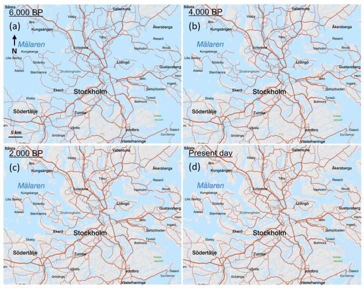
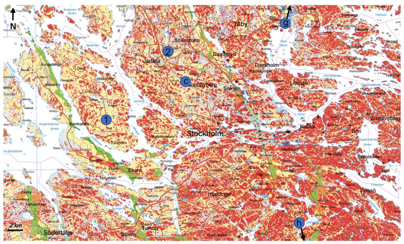
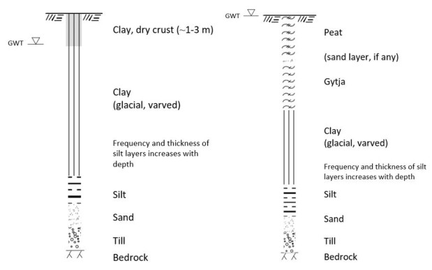
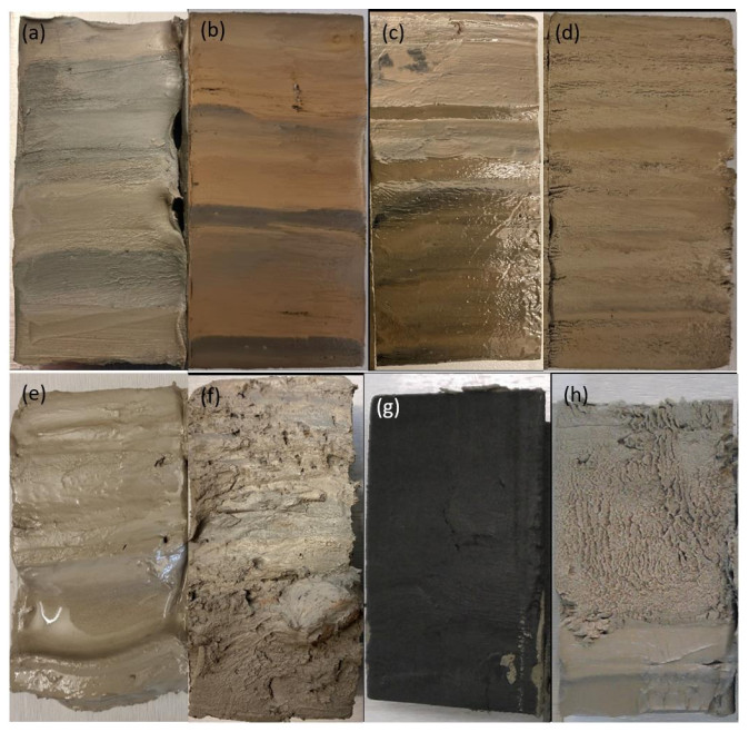
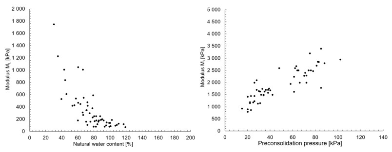
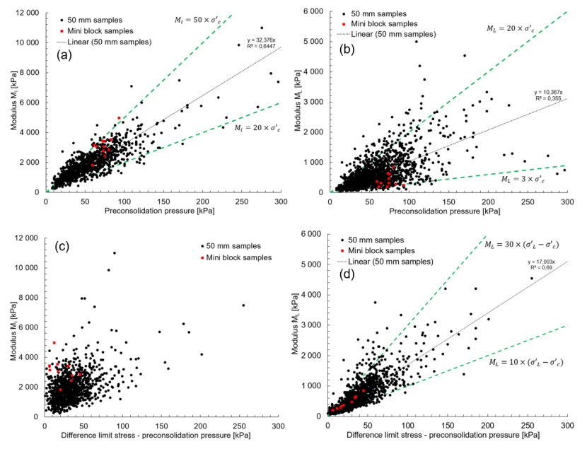
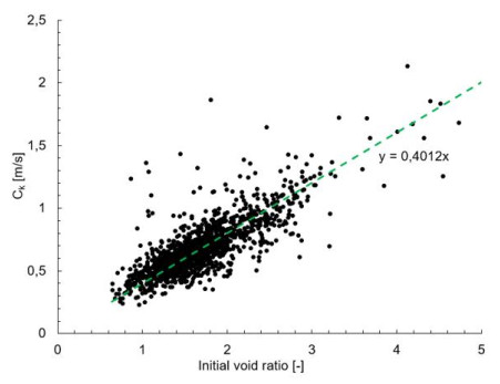
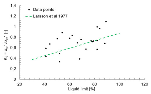
This paper describes the geotechnical characteristics of index and deformation properties of Stockholm clays. These clays exhibit large variations both geographically and with depth. The clays range from highly organic clays with high plasticity to silty clays with low plasticity. First, the geological conditions of the clays are outlined to qualitatively explain the typical soil stratigraphy encountered in the Stockholm area. Second, two large generic databases are presented, containing 3,500 and 1,600 data points, respectively. The data originates from routine testing and constant rate of strain oedometer tests conducted in commercial projects. The data is analyzed and compared with results from high quality block sampling. It is seen that a common feature of the clays are low undrained shear strengths, and consequently low yield stresses and oedometer moduli. Further, several deformation properties such as preconsolidation pressure and several oedometer moduli is shown to depend on the soils natural water content and its plasticity. Differences in sample quality is shown to highly affect some properties, highlighting the importance of quality sampling and handling of samples. Criteria for sample quality for this type of clay is proposed based on the oedometer moduli before and after the preconsolidation pressure. The paper can hopefully work as a useful reference to engineers working on similar soils worldwide.
- clay,
- database,
- index properties,
- deformation properties,
- sample quality
Citation: Solve Hov, David Gaharia. Geotechnical characterization of index and deformation properties of Stockholm clays[J]. AIMS Geosciences, 2023, 9(2): 258-284. doi: 10.3934/geosci.2023015

Related Papers:

Abstract

This paper describes the geotechnical characteristics of index and deformation properties of Stockholm clays. These clays exhibit large variations both geographically and with depth. The clays range from highly organic clays with high plasticity to silty clays with low plasticity. First, the geological conditions of the clays are outlined to qualitatively explain the typical soil stratigraphy encountered in the Stockholm area. Second, two large generic databases are presented, containing 3,500 and 1,600 data points, respectively. The data originates from routine testing and constant rate of strain oedometer tests conducted in commercial projects. The data is analyzed and compared with results from high quality block sampling. It is seen that a common feature of the clays are low undrained shear strengths, and consequently low yield stresses and oedometer moduli. Further, several deformation properties such as preconsolidation pressure and several oedometer moduli is shown to depend on the soils natural water content and its plasticity. Differences in sample quality is shown to highly affect some properties, highlighting the importance of quality sampling and handling of samples. Criteria for sample quality for this type of clay is proposed based on the oedometer moduli before and after the preconsolidation pressure. The paper can hopefully work as a useful reference to engineers working on similar soils worldwide.

References

[1]	Atterberg A (1911) Clays and its water contents and plasticity limits[In Swedish]. Kungliga Lantbruksakademiens Handlingar och Tidskrift 50: 132–158.
[2]	Atterberg A (1912) Consistency of soils[In Swedish]. Kungliga Lantbruksakademiens Handlingar och Tidskrift 51: 93–123.
[3]	Casagrande A (1932) Research on the Atterberg limits of soils. Public Roads 13: 121–136.
[4]	Statens Järnvägar (1922) Swedish State Railways Geotechnical Commission 1914–1922.[In Swedish].
[5]	Hansbo S (1957) A new approach to the determination of the shear strength of clay by the fall-cone test, Swedish Geotechnical Institute, Stockholm.
[6]	Jakobson B (1954) Influence of sampler type and testing method on shear strength of clay samples, Statens Geotekniska Institut, Stockholm.
[7]	Kallstenius T (1958) Mechanical disturbances in clay samples taken with standard piston sampler, Swedish Geotechnical Institute, Stockholm.
[8]	Kallstenius T (1963) Studies on clay samples taken with standard piston sampler, Swedish Geotechnical Institute, Stockholm.
[9]	Cadling L, Odenstad D (1950) The vane borer. An apparatus for determining the shear strength of clay soils directly in the ground, Swedish Geotechnical Institute, Stockholm.
[10]	Bjerrum L, Flodin N (1960) The development of soil mechanics in Sweden, 1900–1925. Géotechnique 10: 1–18. https://doi.org/10.1680/geot.1960.10.1.1 doi: 10.1680/geot.1960.10.1.1
[11]	Lundin S (2000) Geotechnics in Sweden 1920–1945, Swedish Geotechnical Society Report 1.
[12]	Larsson R (1986) Consolidation of soft soils, Swedish Geotechnical Institute.
[13]	Massarsch R, Aronsson S (2014) The Heritage of Swedish Foundation Engineering. Proceedings, DFI/EFFC International Conference on Piling and Deep Foundations, Stockholm, 1031–1054.
[14]	Phoon KK, Ching J, Cao Z (2022) Unpacking data-centric geotechnics. Underground Space 7: 967–989. https://doi.org/10.1016/j.undsp.2022.04.001 doi: 10.1016/j.undsp.2022.04.001
[15]	Phoon KK, Kulhawy FH (1999) Evaluation of geotechnical property variability. Can Geotech J 36: 625–639. https://doi.org/10.1139/t99-039 doi: 10.1139/t99-039
[16]	Phoon KK, Ching J, Shuku T (2022) Challenges in data-driven site characterization. Georisk Assess Manage Risk Eng Syst Geohazards 16: 114–126. https://doi.org/10.1080/17499518.2021.1896005 doi: 10.1080/17499518.2021.1896005
[17]	TC304, TC304 databases. Available from: http://140.112.12.21/issmge/tc304.htm? = 6.
[18]	Swedish Geotechnical Society, Classification and description of soils. Report 1: 2016.
[19]	Swedish Geological Survey, Interactive online maps. 2022. Available from: https://www.sgu.se/om-sgu/nyheter/2022/juni/sgus-strsndforskjutningsmodell-ger-en-bild-av-den-forntida-fordelningen-mellan-hav-och-land/.
[20]	Bjerrum L (1967) Engineering geology of Norwegian normally-consolidated marine clays as related to settlements of buildings. Géotechnique 17: 83–118. https://doi.org/10.1680/geot.1967.17.2.83 doi: 10.1680/geot.1967.17.2.83
[21]	Hov S, Borgström K, Paniagua P (2022) Full-flow CPT tests in a nearshore organic clay. Cone Penetration Test, 452–458.
[22]	Swedish Geological Survey, Description of the geological map Stockholm. 1964.
[23]	Swedish Geotechnical Society, Geotechnical Field Hand Book[In Swedish]. Report 1: 2013.
[24]	Swedish Geotechnical Institute, Swedish Committe on piston samling, Standard piston sampler, Stockholm. 1961.
[25]	Larsson R (1981) Do we obtain undisturbed samples from the standard piston samplers? A comparison with the Laval sampler[In Swedish]. Swedish Geotechnical Insititute.
[26]	Emdal A, Gylland A, Amundsen H, et al. (2016) Mini-block sampler. Can Geotech J 53: 1235–1245. https://doi.org/10.1139/cgj-2015-0628 doi: 10.1139/cgj-2015-0628
[27]	Hov S, Garcia de Herreros C (2020) Comparison of the mini block sampler and the standard piston sampler in a varved East Swedish clay. Report LabMind.
[28]	Karlsson M, Bergström A, Djikstra J (2015) Comparison of the performance of mini-block and piston sampling in high plasticity clays, Technical Report. Chalmers University of Technology, Gothenburg, Sweden.
[29]	Karlsson M, Emdal A, Dijkstra J (2016) Consequences of sample disturbance for predicting long-term settlements in soft clay. Can Geotech J 53. https://doi.org/10.1139/cgj-2016-0129 doi: 10.1139/cgj-2016-0129
[30]	Hov S, Holmén M (2018) The liquid limit[In Swedish]. Swedish Geotechnical Society.
[31]	Hov S, Holmén M (2018) The fall cone test[In Swedish]. Swedish Geotechnical Society.
[32]	Hov S, Prästings A, Persson E, et al. (2021) On Empirical Correlations for Normalised Shear Strengths from Fall Cone and Direct Simple Shear Tests in Soft Swedish Clays. Geotech Geol Eng 39: 4843–4854. https://doi.org/10.1007/s10706-021-01797-w doi: 10.1007/s10706-021-01797-w
[33]	Karlsson R (1981) Consistency Limits in cooperation with the Laboratory Committee of the Swedish Geotechnical Society. Swed Council Build Res, Stockholm, Sweden, Document D6.
[34]	Karlsson R (1961) Suggested improvements in the liquid limit test, with reference to flow properties of remoulded clays. Proc 5th Int Conf Soil Mech Found Eng 1: 171–184.
[35]	Christensen S (2014) Interpretation of field tests, choice of design cuA based on field and laboratory tests[In Norwegian]. Norway's water resources and energy directorate in cooperation with the Norwegian road and railway administrations report no.
[36]	Sällfors G (1975) Preconsolidation pressure of soft, high-plastic clays. Chalmers University of Technology.
[37]	Larsson R, Sällfors G (1986) Automatic Continuous Consolidation Testing in Sweden, Consolidation of Soils: Testing and Evaluation, ASTM STP, 299–328.
[38]	Tidfors M, Sällfors G (1989) Temperature effects on preconsolidation pressure. Geotech Test J 12: 93–97. doi: 10.1520/GTJ10679J
[39]	Boudali M, Leroueil S, Murthy S (1994) Viscous behaviour of natural clays. XⅢ ICSMFE, 411–416.
[40]	Larsson R, Sällfors G (1981) Calculation of settlements in clay[In Swedish]. Väg-och Vattenbyggaren 3: 39–42.
[41]	Paniagua P, L'Heureux JS, Yang SY, et al. (2016) Study on the practices for preconsolidation stress evaluation from oedometer tests. Proc 17th Nord Geotech Meet, 547–555.
[42]	Karlsrud K, Hernandez-Martinez F (2013) Strength and deformation properties of Norwegian clays from laboratory tests on high-quality block samples. Can Geotech J 50: 1273–1293. https://doi.org/10.1139/cgj-2013-0298 doi: 10.1139/cgj-2013-0298
[43]	Janbu N (1963) Soil compressibility as determined by oedometer and triaxial tests. Proc Eur Conf SMFE 1: 19–25.
[44]	Larsson R, Sällfors G, Bengtsson PE, et al. (2007) Shear strength in cohesive soils[In Swedish]. Swedish Geotechnical Institute.
[45]	Berre T, Lunne T, L'Heureux JS (2022) Quantification of sample disturbance for soft, lightly overconsolidated, sensitive clay samples. Can Geotech J 59: 300–303. https://doi.org/10.1139/cgj-2020-0551 doi: 10.1139/cgj-2020-0551
[46]	Ching J, Li DQ, Phoon KK (2016) Statistical characterization of multivariate geotechnical data. Reliability of geotechnical structures in ISO2394, Balkema, CRC Press.
[47]	Bjerrum L (1972) Embankments on soft ground. State of the art report, ASCE Specialty conference on performance of earth and earth-supported structure.
[48]	D'Ignazio M, Phoon KK, Tan SA, et al. (2016) Correlations for undrained shear strength of Finnish soft clays. Can Geotech J 53: 1628–1645. https://doi.org/10.1139/cgj-2016-003 doi: 10.1139/cgj-2016-003
[49]	Ching J, Phoon KK (2012) Modeling parameters of structured clays as a multivariate normal distribution. Can Geotech J 49: 522–545. https://doi.org/10.1139/t2012-015 doi: 10.1139/t2012-015
[50]	Tavenas F, Jean P, Leblond P, et al. (1983) The permeability of natural soils. Part Ⅱ: permeability characteristics. Can Geot J 20: 645–660. https://doi.org/10.1139/t83-073 doi: 10.1139/t83-073
[51]	Larsson R, Bengtsson PE, Eriksson L (1997) Prediction of settlements of embankments on soft, fine-grained soils. Calculation of settlements and their course with time, Swedish Geotechnical Institute.
[52]	Leroueil S, Bouclin G, Tavenas F, et al. (1990) Permeability anisotropy of natural clays as a function of strain. Can Geotech J 27: 568–579. https://doi.org/10.1139/t90-072 doi: 10.1139/t90-072
[53]	Mesri G, Feng T, Ali S, et al. (1994) Permeability characteristics of soft clays. XⅡ ICSMFE, 187–192.
[54]	Larsson R (2008) Properties of soils[In Swedish]. Swedish Geotechnical Institute.
[55]	Larsson R (1977) Basic behaviour of Scandinavian soft clays, Swedish Geotechnical Institute.
[56]	Massarsch R (1979) Lateral earth pressure in normally consolidated clay. Design Parameters in Geotechnical Engineering. Proc 7th Eur Conf Soil Mech Found Eng 2: 245–249.
[57]	L'Heureux JS, Ozkul Z, Lacasse S, et al. (2017) A revised look at the coefficient of earth pressure at rest for Norwegian Clays. NGF Geoteknikkdagen 35.
[58]	DeGroot DJ, Poirier SE, Landon MM (2005) Sample disturbance—soft clays. Studia Geotechnica et Mechanica, Vol. XXVⅡ, 107–120.
[59]	Hight DW, Boese R, Butcher AP, et al. (1992) Disturbance of the Bothkennar clay prior to laboratory testing. Géotechnique 42: 199–217. https://doi.org/10.1680/geot.1992.42.2.199 doi: 10.1680/geot.1992.42.2.199
[60]	Lacasse S, Berre T, Lefevbre G (1985) Block sampling of sensitive clays. Proceedings of the 11th conference on soil mechanics and foundation engineering, San Francisco, CA, 887–892.
[61]	Lunne T, Berre T, Strandvik S (1997) Sample disturbance effects in soft low plastic Norwegian clay. Proceedings of the conference on recent developments in soil and pavement mechanics, Rio de Janeiro, 81–102.
[62]	Clayton CRI, Siddique A (1999) Tube sampling disturbances—fotgotten truths and new perspectives. ICE Geotech Eng 137: 127–135. https://doi.org/10.1680/gt.1999.370302 doi: 10.1680/gt.1999.370302
[63]	Larsson R (2011) SGIs 200 mm diameter block sampler—Undisturbed sampling in fine-grained soils[In Swedish]. Swedish Geotechnical Institute Report 33.
[64]	Löfroth H (2012) Sampling in normal and high sensitive clay—a comparison of results from specimens taken with the SGI large-diameter sampler and the standard piston sampler St Ⅱ. Swedish Geotechnical Institute.
[65]	Andersson M (2022) Personal communication. Swedish Geotechnical Institute.
[66]	Terzaghi K, Peck R, Mesri G (1997) Soil mechanics in engineering practice, Jon Wiley & Sons.
[67]	Donohue S, Long M (2010) Assessment of sample quality in soft clay using shear wave velocity and suction measurements. Géotechnique 60: 883–889. https://doi.org/10.1680/geot.8.T.007.3741 doi: 10.1680/geot.8.T.007.3741

Reader Comments

Your name:*

Email:*
© 2023 the Author(s), licensee AIMS Press. This is an open access article distributed under the terms of the Creative Commons Attribution License (http://creativecommons.org/licenses/by/4.0)