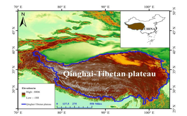
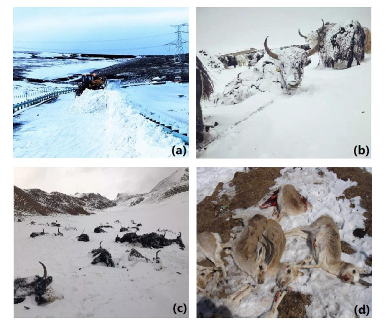
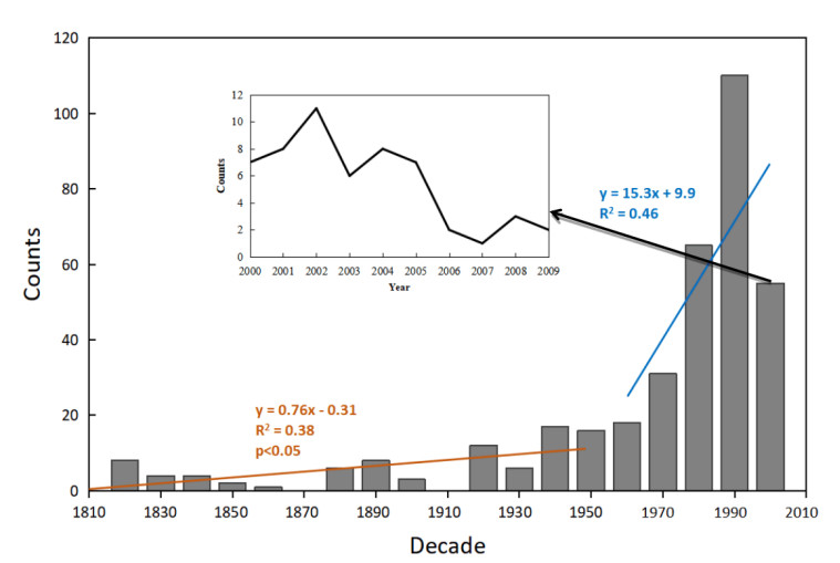
Continuous snowfall caused natural disasters, called snow disasters here, frequently occur on the Qinghai-Tibetan Plateau of China in recent decades, and cause a large number of losses of animal husbandry and human property. However, their long-term changes are poorly known. Here we use historical records to place recent variations of snow disasters under the background of the past 200 years. There are 366 snow disasters events for the 1820–2009 period, of which 230 happen during 1980–2009. In particular, the count of each decadal events since 1980 is larger than any other time during the past two centuries.
Citation: Qi Liu, Le He, Jing Zeng, Yetang Wang. Unprecedented occurrence of snow disasters over the Qinghai-Tibetan Plateau since 1980[J]. AIMS Geosciences, 2021, 7(4): 574-581. doi: 10.3934/geosci.2021033
Continuous snowfall caused natural disasters, called snow disasters here, frequently occur on the Qinghai-Tibetan Plateau of China in recent decades, and cause a large number of losses of animal husbandry and human property. However, their long-term changes are poorly known. Here we use historical records to place recent variations of snow disasters under the background of the past 200 years. There are 366 snow disasters events for the 1820–2009 period, of which 230 happen during 1980–2009. In particular, the count of each decadal events since 1980 is larger than any other time during the past two centuries.

| [1] |
María E, Fernández-Giménez M, Batkhishig B, et al. (2012) Cross-boundary and cross-level dynamics increase vulnerability to severe winter disasters in Mongolia. Global Environ Change 22: 836-851. doi: 10.1016/j.gloenvcha.2012.07.001

|
| [2] |
Li YJ, Ye T, Liu WH, et al. (2018) Linking livestock snow disaster mortality and environmental stressors in the Qinghai-Tibetan Plateau: Quantification based on generalized additive models. Sci Total Environ 625: 87-95. doi: 10.1016/j.scitotenv.2017.12.230
|
| [3] |
Tachiiri K, Shinoda M, Klinkenberg B, et al. (2008) Assessing Mongolian snow disaster risk using livestock and satellite data. J Arid Environ 72: 2251-2263. doi: 10.1016/j.jaridenv.2008.06.015
|
| [4] |
Bocchiola D, Janetti EB, Gorni E, et al. (2008) Regional evaluation of three day snow depth for avalanche hazard mapping in Switzerland. Nat Hazards Earth Syst Sci 8: 685-705. doi: 10.5194/nhess-8-685-2008
|
| [5] |
Delparte D, Jamieson B, Waters N (2008) Statistical runout modeling of snow avalanches using GIS in Glacier National Park, Canada. Cold Reg Sci Technol 54: 183-192. doi: 10.1016/j.coldregions.2008.07.006
|
| [6] |
Yin H, Cao C, Xu M, et al. (2016) Long-term snow disasters during 1982-2012 in the Tibetan Plateau using satellite data. Geomat Nat Haz Risk 8: 466-477. doi: 10.1080/19475705.2016.1238851
|
| [7] |
Nakamura M, Shindo N (2010) Effects of snow cover on the social and foraging behavior of the great tit Parus major. Ecol Res 16: 301-308. doi: 10.1046/j.1440-1703.2001.00397.x
|
| [8] |
Wang W, Liang T, Huang X, et al. (2013) Early warning of snow-caused disasters in pastoral areas on the Tibetan Plateau. Nat Hazards Earth Syst Sci 13: 1411-1425. doi: 10.5194/nhess-13-1411-2013
|
| [9] |
Gao JL, Huang XD, Ma XF, et al. (2017) Snow Disaster Early Warning in Pastoral Areas of Qinghai Province, China. Remote Sens 9: 475. doi: 10.3390/rs9050475
|
| [10] | Yang QY (1995) Geographic museum. Henan: Henan Education Press, 20. Available from: http://hnjybjb.51sole.com/. |
| [11] | Li M, Wang XG, Yang JQ, et al. (2000) Encyclopedia of Yellow River Culture. Sichuan: Sichuan Dictionary Publishing House. |
| [12] | Wen KG, Liu GX (2008) China Meteorological Disaster Ceremony: Tibet. Meteorological Press, Beijing, 34-58. Available from: http://www.qxcbs.com/. |
| [13] | Geng Y (2008) 30 Years of Civil Administration: Qinghai 1978-2008. China Society Press, Beijing, 5. Available from: http://shcbs.mca.gov.cn/. |
| [14] | Shi XH, Li FX, Zhaxi CR, et al. (2006) Snow cover and snow disaster change in Qinghai Province from 1961 to 2004. Chin J Appl Meteorol 3: 376-382. |
| [15] |
Wu JD, Ning L, Yang HJ, et al. (2008) Risk evaluation of heavy snow disasters using BP artificial neural network: the case of Xilingol in Inner Mongolia. Stoch Environ Res Risk Assess 22: 719-725. doi: 10.1007/s00477-007-0181-7
|
| [16] |
Wang SJ, Zhou LY, Wei YQ (2019) Integrated risk assessment of snow disaster over the Qinghai-Tibet Plateau. Geomatics Nat Hazards Risk 10: 740-757. doi: 10.1080/19475705.2018.1543211
|
| [17] | Wen KG, Wang X (2008) China Meteorological Disaster Ceremony: Qinghai. Meteorological Press, Beijing, 169-184. Available from: http://www.qxcbs.com/. |
| [18] | Dong WJ (2004) Yearbook of Meteorological Disasters in China. Beijing: China Meteorological Press, 119-120,123-124. Available from: http://www.qxcbs.com/. |
| [19] | Dong WJ (2005) Yearbook of Meteorological Disasters in China. Beijing: China Meteorological Press, 141-142,146-147. Available from: http://www.qxcbs.com/. |
| [20] | Dong WJ (2006) Yearbook of Meteorological Disasters in China. Beijing: China Meteorological Press, 159-160,164-165. Available from: http://www.qxcbs.com/. |
| [21] | Dong WJ (2007) Yearbook of Meteorological Disasters in China. Beijing: China Meteorological Press, 178-179,183. Available from: http://www.qxcbs.com/. |
| [22] | Xiao ZW (2008) Yearbook of Meteorological Disasters in China. Beijing: China Meteorological Press, 169-170,173-174. Available from: http://www.qxcbs.com/. |
| [23] | Xiao ZW (2009) Yearbook of Meteorological Disasters in China. Beijing: China Meteorological Press, 140-141,145-147. Available from: http://www.qxcbs.com/. |
| [24] | Qinghai Meteorological Bureau, DB63/T 372-2001. Meteorological disaster standard, 2001. Available from: https://wenku.baidu.com/view/267b0a45a8956bec0975e38c.html. |
| [25] | Inspection and Quarantine of the People's Republic of China; Standardization Administration of China, GB/T 20482-2006. General Administration of Quality Supervision, China Meteorological Administration, 2006. |
| [26] | Guo XN, Li L, Liu CH, et al. (2010) Spatial and temporal distribution characteristics of snow disasters in Qinghai Plateau from 1961 to 2008. Clim Change Res 5: 332-337. |
| [27] | Zhang TT, Yan JP, Liao GM, et al. (2014) Spatial and temporal distribution characteristics of snow disasters over Qinghai-Tibet Plateau in recent 51 years. Bull Soil Water Conserv 34: 242-245. |
| [28] | Huang XQ, Tan SY, Ciwang DZ (2018) Changes of snow disasters and their relationship with atmospheric circulation in Tibetan Plateau under the background of climate warming. Plateau Meteorol, 325-332. |
| [29] |
Kuang XX, Jiao JJ (2016) Review on climate change on the Tibetan Plateau during the last half century. J Geophys Res Atmos 121: 3979-4007. doi: 10.1002/2015JD024728
|
| [30] | Song SY, Wuang PX, Du J, et al. (2013) Tibet climate. Beijing: China Meteorological Press, 102-103. |
| [31] |
Deng H, Pepin NC, Chen Y (2017) Changes of snowfall under warming in the Tibetan Plateau. J Geophys Res Atmos 122: 7323-7341. doi: 10.1002/2017JD026524
|
| [32] | Ma WD, Liu FG, Zhou Q, et al. (2020) Characteristics of extreme precipitation over the Tibetan Plateau from 1961 to 2017. J Nat Resour, 3039-3050. |
| [33] |
Ding YJ, Mu CC, Wu TH, et al. (2020) Increasing cryospheric hazards in a warming climate. Earth Sci Rev 213: 103500. doi: 10.1016/j.earscirev.2020.103500
|
| [34] | Long RJ, Liu XY, Cui GX, et al. (2011) Socio-economic changes in pastoral systems on the Tibetan Plateau, Pastoralism and rangeland management on the Tibetan Plateau in the context of climate and global change, Federal Ministry for Economic Cooperation and Development, Berlin, Germany, 239-255. |
| [35] | IPCC (2019) Special Report on the Ocean and Cryosphere in a Changing Climate. Available from: https://www.ipcc.ch/srocc/home/. |
Figures(3) / Tables(1)

Qi Liu, Le He, Jing Zeng, Yetang Wang. Unprecedented occurrence of snow disasters over the Qinghai-Tibetan Plateau since 1980[J]. AIMS Geosciences, 2021, 7(4): 574-581. doi: 10.3934/geosci.2021033


 DownLoad: