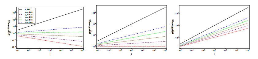
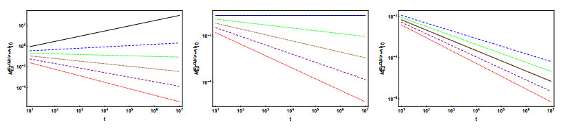
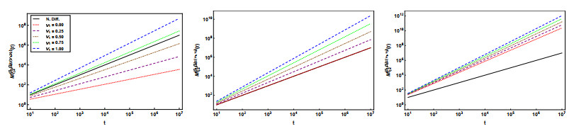
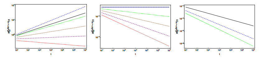
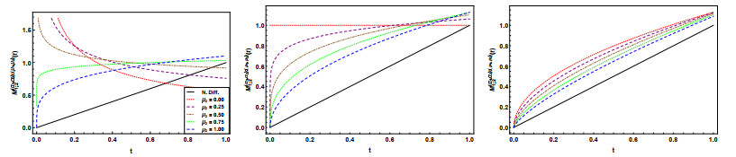
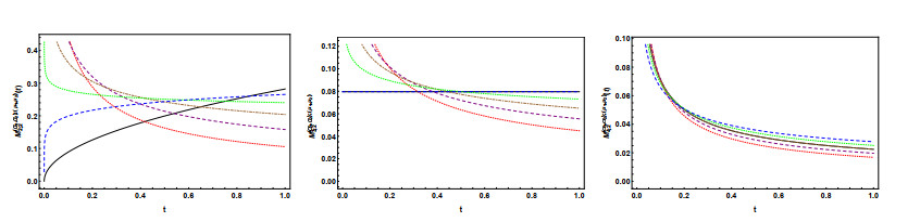
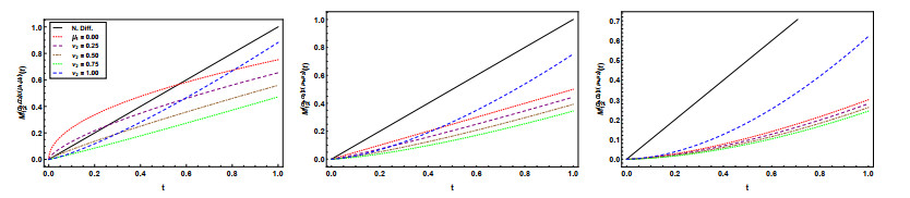
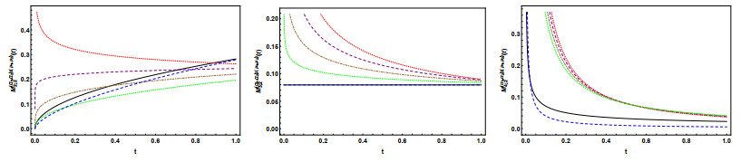
In this paper, we consider the time-fractional telegraph equation of distributed order in higher spatial dimensions, where the time derivative is in the sense of Hilfer, thus interpolating between the Riemann-Liouville and the Caputo fractional derivatives. By employing the techniques of the Fourier, Laplace, and Mellin transforms, we obtain a representation of the solution of the Cauchy problem associated with the equation in terms of convolutions involving functions that are Laplace integrals of Fox H-functions. Fractional moments of the first fundamental solution are computed and for the special case of double-order distributed it is analyzed in detail the asymptotic behavior of the second-order moment, by application of the Tauberian Theorem. Finally, we exhibit plots of the variance showing its behavior for short and long times, and for different choices of the parameters along small dimensions.
Citation: Nelson Vieira, M. Manuela Rodrigues, Milton Ferreira. Time-fractional telegraph equation of distributed order in higher dimensions with Hilfer fractional derivatives[J]. Electronic Research Archive, 2022, 30(10): 3595-3631. doi: 10.3934/era.2022184
In this paper, we consider the time-fractional telegraph equation of distributed order in higher spatial dimensions, where the time derivative is in the sense of Hilfer, thus interpolating between the Riemann-Liouville and the Caputo fractional derivatives. By employing the techniques of the Fourier, Laplace, and Mellin transforms, we obtain a representation of the solution of the Cauchy problem associated with the equation in terms of convolutions involving functions that are Laplace integrals of Fox H-functions. Fractional moments of the first fundamental solution are computed and for the special case of double-order distributed it is analyzed in detail the asymptotic behavior of the second-order moment, by application of the Tauberian Theorem. Finally, we exhibit plots of the variance showing its behavior for short and long times, and for different choices of the parameters along small dimensions.

| [1] |
A. V. Chechkin, R. Gorenflo, I. M. Sokolov, Retarding subdiffusion and accelerating superdiffusion governed by distributed-order fractional diffusion equations, Phys. Rev. E, 66 (2002), 046129. https://doi.org/10.1103/PhysRevE.66.046129 doi: 10.1103/PhysRevE.66.046129

|
| [2] | F. Mainardi, A. Mura, G. Pagnini, R. Gorenflo, Time-fractional diffusion of distributed order, J. Vib. Control, 14 (2008), 1267–1290. https://doi.org/10.1177%2F1077546307087452 |
| [3] |
T. Sandev, A. Chechkin, N. Korabel, H. Kantz, I. M. Sokolov, R. Metzler, Distributed-order diffusion equations and multifractality: Models and solutions, Phys. Rev. E, 92 (2015), 04217. https://doi.org/10.1103/physreve.92.042117 doi: 10.1103/physreve.92.042117
|
| [4] | M. Caputo, Distributed order differential equations modeling dielectric induction and diffusion, Fract. Calc. Appl. Annal., 4 (2001), 421–442. |
| [5] |
A. Ansari, M. Moradi, Exact solutions to some models of distributed-order time fractional diffusion equations via the Fox H functions, ScienceAsia, 39 (2013), 57–66. http://dx.doi.org/10.2306/scienceasia1513-1874.2013.39S.057 doi: 10.2306/scienceasia1513-1874.2013.39S.057
|
| [6] | W. Ding, S. Patnaik, F. Semperlotti, Multiscale nonlocal elasticity: A distributed order fractional formulation, Int. J. Mech. Sci. 226 (2021), 19. https://doi.org/10.1016/j.ijmecsci.2022.107381 |
| [7] |
J. Jia, H. Wang, Analysis of a hidden memory variably distributed-order space-fractional diffusion equation, Appl. Math. Lett., 124 (2022), 107617. https://doi.org/10.1016/j.aml.2021.107617 doi: 10.1016/j.aml.2021.107617
|
| [8] |
J. Jia, X. Zheng, H. Wang, Analysis and fast approximation of a steady-state spatially-dependent distributed-order space-fractional diffusion equation, Fract. Calc. Appl. Anal., 24 (2021), 1477–1506. https://doi.org/10.1515/fca-2021-0062 doi: 10.1515/fca-2021-0062
|
| [9] |
Y. Kumar, V. K. Singh, Computational approach based on wavelets for financial mathematical model governed by distributed order fractional differential equation, Math. Comput. Simul., 190 (2021), 531–569. https://doi.org/10.1016/j.matcom.2021.05.026 doi: 10.1016/j.matcom.2021.05.026
|
| [10] |
M. Naber, Distributed order fractional sub-diffusion, Fractals, 12 (2004), 23–32. https://doi.org/10.1142/S0218348X04002410 doi: 10.1142/S0218348X04002410
|
| [11] | I. M. Sokolov, A. V. Chechkin, J. Klafter, Distributed order fractional kinetics, Acta Physica Polonica, 35 (2004), 1323–1341. |
| [12] | Yu. Luchko, Boundary value problems for the generalized time-fractional diffusion equation of distributed order, Fract. Calc. Appl. Anal., 12(2009), 409–422. |
| [13] |
M. Al-Refai, Yu. Luchko, Analysis of fractional diffusion equations of distributed order: Maximum principles and their applications, Analysis, 36 (2016), 123–133. https://doi.org/10.1515/anly-2015-5011 doi: 10.1515/anly-2015-5011
|
| [14] |
S. Patnaik, F. Semperlotti, Application of variable- and distributed-order fractional operators to the dynamic analysis of nonlinear oscillators, Nonlinear Dyn., 100 (2020), 561–580. https://doi.org/10.1007/s11071-020-05488-8 doi: 10.1007/s11071-020-05488-8
|
| [15] |
R. Gorenflo, Yu. Luchko, M. Stojanović, Fundamental solution of a distributed order time-fractional diffusion-wave equation as probability density, Fract. Calc. Appl. Anal., 16 (2013), 297–316. https://doi.org/10.2478/s13540-013-0019-6 doi: 10.2478/s13540-013-0019-6
|
| [16] | R. Hilfer, Fractional calculus and regular variation in thermodynamics, in Applications of Fractional Calculus in Physics (ed. R. Hilfer), World Scientific, Singapore, (2000), 429–463. |
| [17] |
R. Metzler, J. Klafter, The random walk's guide to anomalous diffusion: A fractional dynamics approach, Phys. Rep., 339 (2000), 1–77. https://doi.org/10.1016/S0370-1573(00)00070-3 doi: 10.1016/S0370-1573(00)00070-3
|
| [18] |
W. Ding, S. Patnaik, S. Sidhardh, F. Semperlotti, Applications of Distributed-Order Fractional Operators: A Review, Entropy, 23 (2021), 110. https://doi.org/10.3390/e23010110 doi: 10.3390/e23010110
|
| [19] |
M. Caputo, M. Fabrizio, The kernel of the distributed order fractional derivatives with an application to complex materials, Fractal Fract., 1 (2017), 13. https://doi.org/10.3390/fractalfract1010013 doi: 10.3390/fractalfract1010013
|
| [20] |
G. Calcagni, Towards multifractional calculus, Front. Phys., 6 (2018), 58. https://doi.org/10.3389/fphy.2018.00058 doi: 10.3389/fphy.2018.00058
|
| [21] | C. F. Lorenzo, T. T. Hartley, Variable order and distributed order fractional operators, Nonlinear Dyn. 29 (2002), 57–98. https://doi.org/10.1023/A:1016586905654 |
| [22] | W. Thomson, On the theory of the electric telegraph, Proc. R. Soc. Lond, Ser. I, 7 (1854), 382–399. https://www.jstor.org/stable/111814 |
| [23] | C. Cattaneo, Sur une forme de l'équation de la chaleur éliminant le paradoxe d'une propagation instantanée, C. R. Acad. Sci., Paris, 246 (1958), 431–433. |
| [24] | W. Hayt, Engineering Electromagnetics, 5th edition, McGraw-Hill, New York, 1989. |
| [25] |
J. Banasiak, R. Mika, Singular perturbed telegraph equations with applications in random walk theory, J. Appl. Stoch. Anal., 11 (1998), 9–28. https://doi.org/10.1155/S1048953398000021 doi: 10.1155/S1048953398000021
|
| [26] |
F. Effenberger, Y. Litvinenko, The diffusion approximation versus the telegraph equation for modeling solar energetic particle transport with adiabatic focusing, Astrophys. J., 783 (2014), 15. https://doi.org/10.1088/0004-637X/783/1/15 doi: 10.1088/0004-637X/783/1/15
|
| [27] | A. Okuko, Application of the telegraph equation to oceanic diffusion: another mathematical model, Technical Report No.69, Chesapeake Bay Institute, Johns Hopkins University, Baltimore, 1971. |
| [28] |
V. H. Weston, S. He, Wave splitting of telegraph equation in $\mathbb{R}$ and its application to inverse scattering, Inverse Probl., 9 (1993), 789–812. https://doi.org/10.1088/0266-5611/9/6/013 doi: 10.1088/0266-5611/9/6/013
|
| [29] |
L. Boyadjiev, Y. Luchko, The neutral-fractional telegraph equation, Math. Model. Nat. Phenom., 12 (2017), 51–67. https://doi.org/10.1051/mmnp/2017064 doi: 10.1051/mmnp/2017064
|
| [30] |
J. Masoliver, Telegraphic transport processes and their fractional generalization: A review and some extensions, Entropy, 23 (2021), 364. https://doi.org/10.3390/e23030364 doi: 10.3390/e23030364
|
| [31] |
E. Orsingher, L. Beghin, Time-fractional telegraph equations and telegraph processes with Brownian time, Probab. Theory Relat. Fields, 128 (2004), 141–160. https://doi.org/10.1007/s00440-003-0309-8 doi: 10.1007/s00440-003-0309-8
|
| [32] |
E. Orsingher, B. Toaldo, Space-time fractional equations and the related stable processes at random time, J. Theor. Probab., 30 (2017), 1–26. https://doi.org/10.1007/s10959-015-0641-9 doi: 10.1007/s10959-015-0641-9
|
| [33] |
R. C. Cascaval, E. C. Eckstein, L. C. Frota, J. A. Goldstein, Fractional telegraph equations, J. Math. Anal. Appl., 276 (2002), 145–159. https://doi.org/10.1016/S0022-247X(02)00394-3 doi: 10.1016/S0022-247X(02)00394-3
|
| [34] |
R. F. Camargo, A. O. Chiacchio, E. C. de Oliveira, Differentiation to fractional orders and the fractional telegraph equation, J. Math. Phys., 49 (2008), 12. https://doi.org/10.1063/1.2890375 doi: 10.1063/1.2890375
|
| [35] |
R. K. Saxena, R. Garra, E. Orsingher, Analytical solution of space-time fractional telegraph-type equations involving Hilfer and Hadamard derivatives, Integr. Transform. Spec. Funct., 27 (2015), 30–42. https://doi.org/10.1080/10652469.2015.1092142 doi: 10.1080/10652469.2015.1092142
|
| [36] |
K. Górska, A. Horzela, E. K. Lenzi, G. Pagnini, T. Sandev, Generalized Cattaneo (telegrapher's) equations in modeling anomalous diffusion phenomena, Phy. Review E, 102 (2020), 13. https://doi.org/10.1103/PhysRevE.102.022128 doi: 10.1103/PhysRevE.102.022128
|
| [37] |
M. Ferreira, M. M. Rodrigues, N. Vieira, Application of the fractional Sturm-Liouville theory to a fractional Sturm-Liouville telegraph equation, Complex Anal. Oper. Theory, 15 (2021), 36. https://doi.org/10.1007/s11785-021-01125-3 doi: 10.1007/s11785-021-01125-3
|
| [38] |
M. Ferreira, M. M. Rodrigues, N. Vieira, First and second fundamental solutions of the time-fractional telegraph equation with Laplace or Dirac operators, Adv. Appl. Clifford Algebr., 28 (2018), 14. https://doi.org/10.1007/s00006-018-0858-7 doi: 10.1007/s00006-018-0858-7
|
| [39] |
M. Ferreira, M. M. Rodrigues, N. Vieira, Fundamental solution of the time-fractional telegraph Dirac operator, Math. Methods Appl. Sci., 40 (2017), 7033–7050. https://doi.org/10.1002/mma.4511 doi: 10.1002/mma.4511
|
| [40] |
M. Ferreira, M. M. Rodrigues, N. Vieira, Fundamental solution of the multi-dimensional time fractional telegraph equation, Fract. Calc. Appl. Anal., 20 (2017), 868–894. https://doi.org/10.1515/fca-2017-0046 doi: 10.1515/fca-2017-0046
|
| [41] |
M. D'Ovidio, E. Orsingher, B. Toaldo, Time-changed processes governed by space-time fractional telegraph equations, Stoch. Anal. Appl., 32 (2014), 1009–1045. https://doi.org/10.1080/07362994.2014.962046 doi: 10.1080/07362994.2014.962046
|
| [42] | J. Masoliver, K. Lindenberg, Two-dimensional telegraphic processes and their fractional generalizations, Phys. Rev. E, 101 (2020). https://doi.org/10.1103/PhysRevE.101.012137 |
| [43] | J. Masoliver, Three-dimensional telegrapher's equation and its fractional generalization, Phys. Rev. E, 96 (2017). https://link.aps.org/doi/10.1103/PhysRevE.96.022101 |
| [44] | J. Masoliver, Fractional telegrapher's equation from fractional persistent random walks, Phys. Rev. E, 93 (2016). https://link.aps.org/doi/10.1103/PhysRevE.93.052107 |
| [45] |
J. Masoliver, J. M. Porrà, G. H. Weiss, Some two and three-dimensional persistent random walks, Phys. A: Stat. Mech. Appl., 193 (1993), 469–482. https://doi.org/10.1016/0378-4371(93)90488-P doi: 10.1016/0378-4371(93)90488-P
|
| [46] | N. Vieira, M. M. Rodrigues, M. Ferreira, Time-fractional telegraph equation of distributed order in higher dimensions, Commun. Nonlinear Sci. Numer. Simulat., 102 (2021). https://doi.org/10.1016/j.cnsns.2021.105925 |
| [47] | R. Hilfer, Applications of Fractional Calculus in Physics, World Scientific, Singapore, 2000. |
| [48] | R. Hilfer, Threefold introduction to fractional derivatives, Chapter 2, in: Anomalous Transport: Foundations and Applications (eds. R. Klages, G.Radons and I.M. Sokolov). Weinheim: Wiley-VCH, (2008), 17–74. |
| [49] |
R. Hilfer, Experimental evidence for fractional time evolution in glass forming materials, Chem. Phys., 284 (2002), 399–408. https://doi.org/10.1016/S0301-0104(02)00670-5 doi: 10.1016/S0301-0104(02)00670-5
|
| [50] | R. Hilfer, Y. Luchko, Z. Tomovski, Operational method for the solution of fractional differential equations with generalized Riemann-Liouville fractional derivatives, Fract. Calc. Appl. Anal., 12 (2009), 299–318. |
| [51] |
T. Sandev, Z. Tomovski, B. Crnkovic, Generalized distributed order diffusion equations with composite time fractional derivative, Comput. Math. Appl., 73 (2017), 1028–1040. https://doi.org/10.1016/j.camwa.2016.07.009 doi: 10.1016/j.camwa.2016.07.009
|
| [52] |
R. K. Saxena, A. M. Mathai, H. J. Haubold, Space–time fractional reaction-diffusion equations associated with a generalized Riemann–Liouville fractional derivative, Axioms, 3 (2014), 320–334. https://doi.org/10.3390/axioms3030320 doi: 10.3390/axioms3030320
|
| [53] | R. K. Saxena, Z. Tomovski, T. Sandev, Fractional Helmholtz and fractional wave equations with Riesz-Feller and generalized Riemann-Liouville fractional derivatives, Eur. J. Pure Appl. Math., 7 (2014), 312–334. http://www.ejpam.com/index.php/ejpam/article/view/2176 |
| [54] |
Z. Tomovski, Generalized Cauchy type problems for nonlinear fractional differential equations with composite fractional derivative operator, Nonlinear Anal., 75 (2012), 3364–3384. https://doi.org/10.1016/j.na.2011.12.034 doi: 10.1016/j.na.2011.12.034
|
| [55] |
Z. Tomovski, T. Sandev, R. Metzler, J. Dubbeldam, Generalized space-time fractional diffusion equation with composite fractional time derivative, Phys. A., 391 (2012), 2527–2542. 10.1016/j.physa.2011.12.035 doi: 10.1016/j.physa.2011.12.035
|
| [56] |
Z. Tomovski, T. Sandev, Distributed-order wave equations with composite time fractional derivative, Int. J. Comput. Math., 95 (2018), 1100–1113. https://doi.org/10.1080/00207160.2017.1366465 doi: 10.1080/00207160.2017.1366465
|
| [57] | A. A. Kilbas, H. M. Srivastava, J. J. Trujillo, Theory and Applications of Fractional Differential Equations, North-Holland Mathematics Studies, Elsevier, Amsterdam, 2006. |
| [58] | S. G. Samko, A. A. Kilbas, O. I. Marichev, Fractional Integrals and Derivatives: Theory and Applications, Gordon and Breach, New York, 1993. |
| [59] | E. C. Titchmarsh, Introduction to the Theory of Fourier Integrals, Clarendon Press, Oxford, 1937. |
| [60] | A. A. Kilbas, M. Saigo, H-transforms. Theory and applications, Analytical Methods and Special Functions, Chapman & Hall/CRC, Boca Raton, 2004. |
| [61] | R. Gorenflo, A. A. Kilbas, F. Mainardi, S. V. Rogosin, Mittag-Leffler Functions, Related Topics and Applications, 2nd extended and updated edition, Springer Monographs in Mathematics, Springer, Berlin, 2020. |
| [62] |
M. Ferreira, N. Vieira, Fundamental solutions of the time fractional diffusion-wave and parabolic Dirac operators, J. Math. Anal. Appl., 447 (2017), 329–353. https://doi.org/10.1016/j.jmaa.2016.08.052 doi: 10.1016/j.jmaa.2016.08.052
|
| [63] | A. P. Prudnikov, Y. A. Brychkov, O. I. Marichev, Integrals and series. Volume 5: Inverse Laplace transforms, Gordon and Breach Science Publishers, New York etc., 1992. |
| [64] |
R. Garrapa, Numerical evaluation of two and three parameter Mittag-Leffler functions, SIAM J. Numer. Anal., 53 (2015), 1350–1369. https://doi.org/10.1137/140971191 doi: 10.1137/140971191
|
| [65] | N. Vieira, M. Ferreira, M. M. Rodrigues, Time-fractional telegraph equation with $\psi$-Hilfer derivatives, Comput. Appl. Math., 41 (2022). |
Figures(8)
Nelson Vieira, M. Manuela Rodrigues, Milton Ferreira. Time-fractional telegraph equation of distributed order in higher dimensions with Hilfer fractional derivatives[J]. Electronic Research Archive, 2022, 30(10): 3595-3631. doi: 10.3934/era.2022184


 DownLoad: