Long-term exposure to pollution from particulate matter in palm oil mills can result in chronic respiratory diseases, cardiovascular diseases and mortality. Particulate matter with a size of less than 2.5 μm (PM2.5) has a greater impact than one with a size of 10 μm. The current PM cleaning equipment in palm oil mills consists of cyclones that are incapable of optimally filtering PM2.5. For this reason, it is necessary to design cyclone applications for fine particle separation in palm oil mills. Normal cyclones are incapable of segregating particles smaller than 2.5 μm. This study's objective was to design a cyclone with a filter on the vortex detector. These cyclones are utilized in PM2.5 fine particle filtration systems. Using computational fluid dynamics, cyclone performance is analyzed in terms of removal efficiency and pressure decrease. The research was conducted utilizing the Reynolds tress model with varying inlet velocities of 10, 15, 20, 25 and 30 meters per second. The filter is composed of boiler bottom ash refuse from palm oil mills; 0.310 meters is the height of the filter bed inserted in the vortex finder. The obtained results demonstrated that the PM2.5 removal efficiency reached 98%, while the pressure decrease was only 93 Pa greater than that of conventional cyclones. Thereby, cyclone designs with bottom ash filters can be used to filter fine particulate matter, particularly particles smaller than 2.5 μm.
Citation: Novi Sylvia, Husni Husin, Abrar Muslim, Yunardi, Aden Syahrullah, Hary Purnomo, Rozanna Dewi, Yazid Bindar. Design and performance of a cyclone separator integrated with a bottom ash bed for the removal of fine particulate matter in a palm oil mill: A simulation study[J]. AIMS Environmental Science, 2023, 10(3): 341-355. doi: 10.3934/environsci.2023020
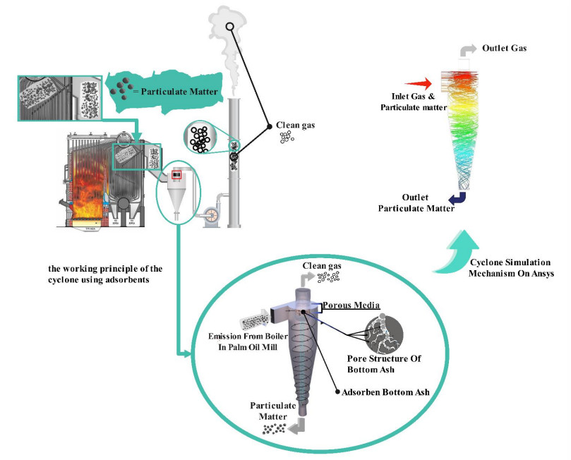
Long-term exposure to pollution from particulate matter in palm oil mills can result in chronic respiratory diseases, cardiovascular diseases and mortality. Particulate matter with a size of less than 2.5 μm (PM2.5) has a greater impact than one with a size of 10 μm. The current PM cleaning equipment in palm oil mills consists of cyclones that are incapable of optimally filtering PM2.5. For this reason, it is necessary to design cyclone applications for fine particle separation in palm oil mills. Normal cyclones are incapable of segregating particles smaller than 2.5 μm. This study's objective was to design a cyclone with a filter on the vortex detector. These cyclones are utilized in PM2.5 fine particle filtration systems. Using computational fluid dynamics, cyclone performance is analyzed in terms of removal efficiency and pressure decrease. The research was conducted utilizing the Reynolds tress model with varying inlet velocities of 10, 15, 20, 25 and 30 meters per second. The filter is composed of boiler bottom ash refuse from palm oil mills; 0.310 meters is the height of the filter bed inserted in the vortex finder. The obtained results demonstrated that the PM2.5 removal efficiency reached 98%, while the pressure decrease was only 93 Pa greater than that of conventional cyclones. Thereby, cyclone designs with bottom ash filters can be used to filter fine particulate matter, particularly particles smaller than 2.5 μm.

| [1] |
Burnett RT, Smith-Doiron M, Stieb D, et al. (1999) Effects of particulate and gaseous air pollution on cardiorespiratory hospitalizations. Arch Environ Health 54: 130–139. https://doi.org/10.1080/00039899909602248 doi: 10.1080/00039899909602248

|
| [2] |
Zanobetti A, Schwartz J (2009) The effect of fine and coarse particulate air pollution on mortality: A national analysis. Environ Health Perspect 117: 898–903. https://doi.org/10.1289/ehp.0800108 doi: 10.1289/ehp.0800108
|
| [3] |
Cheng BJ, Zhou Y, Ma Y, et al. (2022) Association between atmospheric particulate matter and emergency room visits for cerebrovascular disease in Beijing, China. J Environ Health Sci Eng 20: 293–303. https://doi.org/10.1007/s40201-021-00776-w doi: 10.1007/s40201-021-00776-w
|
| [4] | Syahirah MM, Rashid M, Nor Ruwaida J (2016) Total particulate matter, pm10, pm2.5 emissions from palm oil mill boiler. Jurnal Teknologi 78: 6–11. |
| [5] |
Chong WC, Rashid M, Ramli M, et al. (2014) Effect of flue gas recirculation on multi-cyclones performance in reducing particulate emission from palm oil mill boiler. Particul Sci Technol 32: 291–297. https://doi.org/10.1080/02726351.2013.856360 doi: 10.1080/02726351.2013.856360
|
| [6] |
Bogodage SG, Leung AYT (2015) CFD simulation of cyclone separators to reduce air pollution. Powder Technol 286: 488–506. https://doi.org/10.1016/j.powtec.2015.08.023 doi: 10.1016/j.powtec.2015.08.023
|
| [7] |
Elsayed K, Lacor C (2012) Modeling and Pareto optimization of gas cyclone separator performance using RBF type artificial neural networks and genetic algorithms. Powder Technol 217: 84–99. https://doi.org/10.1016/j.powtec.2011.10.015 doi: 10.1016/j.powtec.2011.10.015
|
| [8] |
Funk PA, Elsayed K, Yeater KM, et al. (2015) Could cyclone performance improve with reduced inlet velocity? Powder Technol 280: 211–218. https://doi.org/10.1016/j.powtec.2015.04.026 doi: 10.1016/j.powtec.2015.04.026
|
| [9] |
Park D, Go JS (2020) Design of cyclone separator critical diameter model based on machine learning and CFD. Processes 8: 1521. https://doi.org/10.3390/pr8111521 doi: 10.3390/pr8111521
|
| [10] |
Pandey S, Brar LS (2022) On the performance of cyclone separators with different shapes of the conical section using CFD. Powder Technol 407: 117629. https://doi.org/10.1016/j.powtec.2022.117629 doi: 10.1016/j.powtec.2022.117629
|
| [11] |
Pandey SI, Saha O, Prakash T, et al. (2022) CFD Investigations of cyclone separators with different cone heights and shapes. Appl Sci 12: 4904. https://doi.org/10.3390/app12104904 doi: 10.3390/app12104904
|
| [12] |
Youn JS, Han S, Yi JS, et al. (2021) Development of PM10 and PM2.5 cyclones for small sampling ports at stationary sources: Numerical and experimental study. Environ Res 193: 110507. https://doi.org/10.1016/j.envres.2020.110507 doi: 10.1016/j.envres.2020.110507
|
| [13] |
Duran JZ, Caldona, EB (2020) Design of an activated carbon equipped-cyclone separator and its performance on particulate matter removal. Particul Sci Technol 38: 694–702. https://doi.org/10.1080/02726351.2019.1607637 doi: 10.1080/02726351.2019.1607637
|
| [14] |
Hayashi T, Lee TG, Hazelwood M, et al. (2000) Characterization of activated carbon fiber filters for pressure drop, submicrometer particulate collection, and mercury capture. J Air Waste Manag Assoc 50: 922–929. https://doi.org/10.1080/10473289.2000.10464136 doi: 10.1080/10473289.2000.10464136
|
| [15] |
Shanmuganathan S, Johir MA, Nguyen TV, et al. (2015) Experimental evaluation of microfiltration–granular activated carbon (MF–GAC)/nano filter hybrid system in high quality water reuse. J Membr Sci 476: 1–9. https://doi.org/10.1016/j.memsci.2014.11.009 doi: 10.1016/j.memsci.2014.11.009
|
| [16] |
Ma L, He M, Fu P, et al. (2020) Adsorption of volatile organic compounds on modified spherical activated carbon in a new cyclonic fluidized bed. Sep Purif Technol 235: 1–11. https://doi.org/10.1016/j.seppur.2019.116146 doi: 10.1016/j.seppur.2019.116146
|
| [17] |
Hamzah MH, Ahmad Asri MF, Che Man H, et al. (2019) Prospective application of palm oil mill boiler ash as a biosorbent: effect of microwave irradiation and palm oil mill effluent decolorization by adsorption. Int J Environ Res Public Health 16: 3453. https://doi.org/10.3390/ijerph16183453 doi: 10.3390/ijerph16183453
|
| [18] |
Sylvia N, Fitriani F, Dewi R, et al. (2021) Characterization of bottom ash waste adsorbent from palm oil plant boiler burning process to adsorb carbon dioxide in a fixed bed column. Indones J Chem 21: 1454–1462. https://doi.org/10.22146/ijc.66509 doi: 10.22146/ijc.66509
|
| [19] | Awang HB, Al-Mulali MZ (2018) The Inclusion of Palm Oil Ash Biomass Waste in Concrete: A Literature Review." In (Ed.), Palm Oil. IntechOpen. https://doi.org/10.5772/intechopen.76632 |
| [20] |
Promraksa A, Rakmak N (2020) Biochar production from palm oil mill residues and application of the biochar to adsorb carbon dioxide. Heliyon 6: e04019. https://doi.org/10.1016/j.heliyon.2020.e04019 doi: 10.1016/j.heliyon.2020.e04019
|
| [21] |
Igwe JC, Arukwe U, Anioke SN (2013) Isotherm and kinetic studies of residual oil adsorption from palm oil mill effluent (pome) using boiler fly ash. Environ Eng Manag J 12: 417–427. https://doi.org/10.30638/eemj.2013.052 doi: 10.30638/eemj.2013.052
|
| [22] | Fluent Theory Guide (2016) Fluent Inc.: Canonsburg, PA, USA. |
| [23] | Wilcox DC (1994). Turbulence modeling for CFD; DCW Industries, Inc.: La Cañada Flintridge, CA, USA. |
| [24] |
Liu X, Shen H, Nie X (2019) Study on the filtration performance of the baghouse filters for ultra-low emission as a function of filter pore size and fiber diameter. Int J Environ Res Public Health 16: 247. http://dx.doi.org/10.3390/ijerph16020247 doi: 10.3390/ijerph16020247
|


Figures(13) / Tables(3)

Novi Sylvia, Husni Husin, Abrar Muslim, Yunardi, Aden Syahrullah, Hary Purnomo, Rozanna Dewi, Yazid Bindar. Design and performance of a cyclone separator integrated with a bottom ash bed for the removal of fine particulate matter in a palm oil mill: A simulation study[J]. AIMS Environmental Science, 2023, 10(3): 341-355. doi: 10.3934/environsci.2023020


 DownLoad: