Temperature prediction and analysis based on improved GA-BP neural network

Ling Zhang; Xiaoqi Sun; Shan Gao; Ling Zhang; Xiaoqi Sun; Shan Gao

doi:10.3934/environsci.2022042

AIMS Environmental Science

2022, Volume 9, Issue 5: 735-753. doi: 10.3934/environsci.2022042

Previous Article Next Article

Research article

Temperature prediction and analysis based on improved GA-BP neural network

School of Mathematics and Statistics, Qingdao University, Shinan District, Qingdao, Shandong, China

Received: 14 June 2022 Revised: 21 September 2022 Accepted: 10 October 2022 Published: 31 October 2022

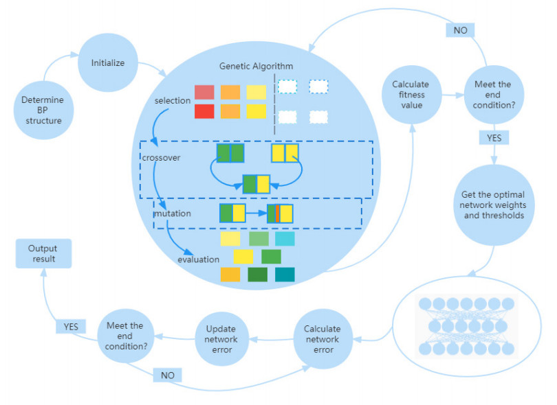
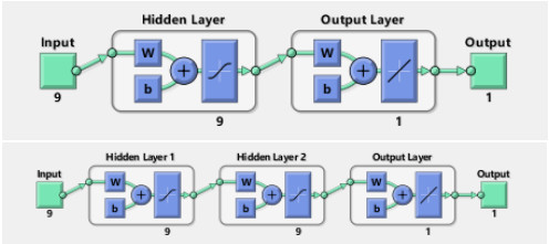
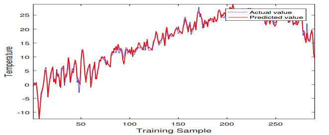
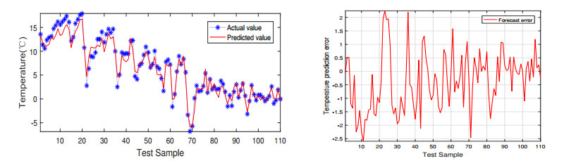
In order to predict the temperature change of Laoshan scenic area in Qingdao more accurately, a new back propagation neural network (BPNN) prediction model is proposed in this study. Temperature change affects our lives in various ways. The challenge that neural networks tend to fall into local optima needs to be addressed to increase the accuracy of temperature prediction. In this research, we used an improved genetic algorithm (GA) to optimize the weights and thresholds of BPNN to solve this problem. The prediction results of BPNN and GA-BPNN were compared, and the prediction results showed that the prediction performance of GA-BPNN was much better. Furthermore, a screening test experiment was conducted using GA-BPNN for multiple classes of meteorological parameters, and a smaller number of parameter sets were identified to simplify the prediction inputs. The values of running time, root mean square error, and mean absolute error of GA-BPNN are better than those of BPNN through the calculation and analysis of evaluation metrics. This study will contribute to a certain extent to improve the accuracy and efficiency of temperature prediction in the Laoshan landscape.
- temperature prediction,
- genetic algorithm,
- BP neural network,
- neural network optimization
Citation: Ling Zhang, Xiaoqi Sun, Shan Gao. Temperature prediction and analysis based on improved GA-BP neural network[J]. AIMS Environmental Science, 2022, 9(5): 735-753. doi: 10.3934/environsci.2022042

Related Papers:

Abstract

In order to predict the temperature change of Laoshan scenic area in Qingdao more accurately, a new back propagation neural network (BPNN) prediction model is proposed in this study. Temperature change affects our lives in various ways. The challenge that neural networks tend to fall into local optima needs to be addressed to increase the accuracy of temperature prediction. In this research, we used an improved genetic algorithm (GA) to optimize the weights and thresholds of BPNN to solve this problem. The prediction results of BPNN and GA-BPNN were compared, and the prediction results showed that the prediction performance of GA-BPNN was much better. Furthermore, a screening test experiment was conducted using GA-BPNN for multiple classes of meteorological parameters, and a smaller number of parameter sets were identified to simplify the prediction inputs. The values of running time, root mean square error, and mean absolute error of GA-BPNN are better than those of BPNN through the calculation and analysis of evaluation metrics. This study will contribute to a certain extent to improve the accuracy and efficiency of temperature prediction in the Laoshan landscape.

References

[1]	Khaniani AS, Motieyan H, Mohammadi A (2021) Rainfall forecast based on GPS PWV together with meteorological parameters using neural network models. J Atmos Sol-Terr Phy 214: 105533. http://doi.org/10.1016/J.JASTP.2020.105533 doi: 10.1016/J.JASTP.2020.105533
[2]	Huang H, Zhang JX, Song YP, et al. (2016) Prediction for quarterly precipitation in Xinjiang based on fuzzy time series prediction model. Fuzzy Syst Math 30: 176–182.
[3]	Lee J, Kim CG, Lee J E, et al. (2018) Application of artificial neural networks to rainfall forecasting in the Geum River basin, Korea. Water 10: 1448. http://doi.org/10.3390/w10101448 doi: 10.3390/w10101448
[4]	Liu Y, Zhao QZ, Yao WQ, et al. (2019) Short-term rainfall forecast model based on the improved BP–NN algorithm. Sci Rep 9: 19751. http://doi.org/10.1038/s41598-019-56452-5 doi: 10.1038/s41598-019-56452-5
[5]	Guan ZM, Tian ZY, Xu YS, et al. (2016) Rain fall predict and comparing research based on Arcgis and BP neural network. 2016 3rd international conference on materials engineering, manufacturing technology and control, 1509–1514. http://doi.org/10.2991/icmemtc-16.2016.291 doi: 10.2991/icmemtc-16.2016.291
[6]	Peng YZ, Gong DQ, Deng CY, et al. (2022) An automatic hyperparameter optimization DNN model for precipitation prediction. Appl Intell 52: 2703–2719. http://doi.org/10.1007/S10489-021-02507-Y doi: 10.1007/S10489-021-02507-Y
[7]	Cho D, Yoo C, Son B, et al. (2022) A novel ensemble learning for post-processing of NWP Model's next-day maximum air temperature forecast in summer using deep learning and statistical approaches. Weather Clim Extreme 35: 100410. http://doi.org/10.1016/J.WACE.2022.100410 doi: 10.1016/J.WACE.2022.100410
[8]	Shi JH, Yu J, Yang JK, et al. (2022) Time series surface temperature prediction based on cyclic evolutionary network model for complex sea area. Future Internet 14: 96. http://doi.org/10.3390/FI14030096 doi: 10.3390/FI14030096
[9]	Song TY, Huang GH, Wang GQ, et al. (2022) Bayesian model averaging of the RegCM temperature projections: A Canadian case study. J Water Clim Change 13: 771–785. http://doi.org/10.2166/WCC.2021.393 doi: 10.2166/WCC.2021.393
[10]	Gupta S, Tripathi M, Grover J (2022) Hybrid optimization and deep learning based intrusion detection system. Comput Electr Eng 100: 107876. http://doi.org/10.1016/J.COMPELECENG.2022.107876 doi: 10.1016/J.COMPELECENG.2022.107876
[11]	Lei YS, Cai XJ, Wang W (2018) Application research of BP neural network optimized by genetic algorithm in multi-model ensemble forecasr about ground temperature. J Meteorol Sci 38: 806–814.
[12]	Yao C, Jin L, Huang MC, et al. (2007) An experiment with methods of forecasting tropical cyclones intensity base on combination of the genetic algorithm and artificial neural network. Acta Oceanol Sin 29: 11–19.
[13]	Wu JS (2016) Hybrid optimization algorithm to combine neural network for rainfall-runoff modeling. Int J Comput Intell 15: 1650015. http://doi.org/10.1142/S1469026816500152 doi: 10.1142/S1469026816500152
[14]	Sun T, Chen YD, Meng DM, et al. (2021) Background error covariance statistics of hydrometeor control variables based on gaussian transform. Adv Atmos Sci 38: 831–844. http://doi.org/10.1007/S00376-021-0271-3 doi: 10.1007/S00376-021-0271-3
[15]	Tang SZ, Li MJ, Wang FL, et al. (2020) Fouling potential prediction and multi-objective optimization of a flue gas heat exchanger using neural networks and genetic algorithms. Int J Heat Mass Tran 152: 119488. http://doi.org/10.1016/j.ijheatmasstransfer.2020.119488 doi: 10.1016/j.ijheatmasstransfer.2020.119488
[16]	Liu CH, Yang L, Deng H, et al. (2019) Prediction of ammonia concentration in piggery based on ARIMA and BP neural network. China Environ Sci 39: 2320–2327. http://doi.org/10.19674/j.cnki.issn1000-6923.2019.0276 doi: 10.19674/j.cnki.issn1000-6923.2019.0276
[17]	Xie YQ, Ishidal Y, Hu JL, et al. (2022) A backpropagation neural network improved by a genetic algorithm for predicting the mean radiant temperature around buildings within the long-term period of the near future. Build Simul 15: 473–492. http://doi.org/10.1007/S12273-021-0823-6 doi: 10.1007/S12273-021-0823-6

Reader Comments

Your name:*

Email:*
© 2022 the Author(s), licensee AIMS Press. This is an open access article distributed under the terms of the Creative Commons Attribution License (http://creativecommons.org/licenses/by/4.0)