Model for measuring concentration ratio distribution of a dish concentrator using moonlight as a precursor for solar tower flux mapping

Minghuan Guo; Hao Wang; Zhifeng Wang; Xiliang Zhang; Feihu Sun; Nan Wang; Minghuan Guo; Hao Wang; Zhifeng Wang; Xiliang Zhang; Feihu Sun; Nan Wang

doi:10.3934/energy.2021034

AIMS Energy

2021, Volume 9, Issue 4: 727-754. doi: 10.3934/energy.2021034

Previous Article Next Article

Research article Special Issues

Model for measuring concentration ratio distribution of a dish concentrator using moonlight as a precursor for solar tower flux mapping

1.
Institute of Electrical Engineering, Chinese Academy of Sciences, No.6 Beiertiao, Zhongguancun, Haidian District, Beijing, 100190, China
2.
School of Engineering Science, University of Chinese Academy of Sciences, No. 380, Huaibei Town, Huairou District, Beijing, 101408, China
3.
Beijing Engineering Research Center of Solar Thermal Power, No.6 Beiertiao, Zhongguancun, Haidian District, Beijing, 100190, China
4.
State Grid Shanxi Electric Power Research Institute, No. 6, Qingnian Road, Yingze District, Taiyuan City, Shanxi Province, 030000, China

Received: 09 February 2021 Accepted: 08 June 2021 Published: 16 June 2021

Measuring solar flux distribution (also called flux mapping) of a large receiver is quite challenging. Lunar flux mapping measures the illuminance distribution on the receiver aperture and the direct normal lunar illuminance during moonlight concentration experiments to determine the concentration ratio distribution (CRD). This paper presents a new lunar flux mapping model to extend the applicability to parts of the lunar cycle where the moon is not full. A dish concentrator with a similar concentration ratio to a tower concentrator was built in Beijing and used for lunar flux mapping experiments. A general method of backward ray tracing with effective sun/moon shapes for simulation of CRD is developed. The moonshape image and the normalized error image are convolved in two dimensions using the Fast Fourier Transform to give the effective moon shape image. Several optical simulations and moonlight concentration measurements on the concentrator show good similarity in the effects of changes in light source shape between solar and lunar CRD images. This model recognizes the potential of a solar concentrator to enhance the similarity between the solar CRD and a lunar CRD and that the residual differences can be compensated to some extent by using the smoothing filtering of the lunar CRD image to approximate the expected solar CRD image. The cosine similarity between lunar and solar CRDs is a function of the cosine similarity between the corresponding light source shapes, which can be derived from the dish concentrator and shows promise for application to a large solar tower system.
- solar tower concentrator,
- moonlight concentration,
- flux mapping,
- solar dish,
- concentration ratio distribution,
- smoothing filter,
- cosine similarity
Citation: Minghuan Guo, Hao Wang, Zhifeng Wang, Xiliang Zhang, Feihu Sun, Nan Wang. Model for measuring concentration ratio distribution of a dish concentrator using moonlight as a precursor for solar tower flux mapping[J]. AIMS Energy, 2021, 9(4): 727-754. doi: 10.3934/energy.2021034

Related Papers:

Abstract

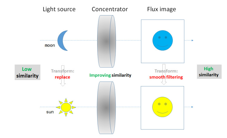
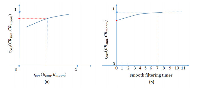
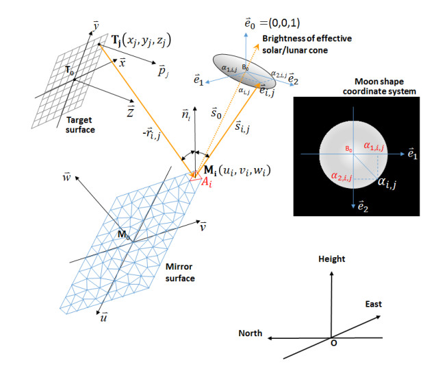
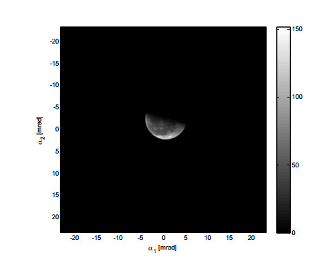
Measuring solar flux distribution (also called flux mapping) of a large receiver is quite challenging. Lunar flux mapping measures the illuminance distribution on the receiver aperture and the direct normal lunar illuminance during moonlight concentration experiments to determine the concentration ratio distribution (CRD). This paper presents a new lunar flux mapping model to extend the applicability to parts of the lunar cycle where the moon is not full. A dish concentrator with a similar concentration ratio to a tower concentrator was built in Beijing and used for lunar flux mapping experiments. A general method of backward ray tracing with effective sun/moon shapes for simulation of CRD is developed. The moonshape image and the normalized error image are convolved in two dimensions using the Fast Fourier Transform to give the effective moon shape image. Several optical simulations and moonlight concentration measurements on the concentrator show good similarity in the effects of changes in light source shape between solar and lunar CRD images. This model recognizes the potential of a solar concentrator to enhance the similarity between the solar CRD and a lunar CRD and that the residual differences can be compensated to some extent by using the smoothing filtering of the lunar CRD image to approximate the expected solar CRD image. The cosine similarity between lunar and solar CRDs is a function of the cosine similarity between the corresponding light source shapes, which can be derived from the dish concentrator and shows promise for application to a large solar tower system.

References

[1]	Ballestrín J, Burgess G, Cumpston J (2012) Heat flux and temperature measurement technologies for concentrating solar power(CSP), In: Lovegrove, K and Stein, W, Concentrating solar power technology: Principles, developments and applications, 1 Eds., Cambridge: Woodhead Publishing Limited, 577-593.
[2]	Osuna R, Morillo R, Jiménez JM, et al. (2006) Control and operation strategies in PS10 solar plant. 13th SolarPACES Conference.
[3]	Ballestrín J (2002) A non-water-cooled heat flux measurement system under concentrated solar radiation conditions. Sol Energy 73: 159-168. doi: 10.1016/S0038-092X(02)00046-4
[4]	Ballestrín J, Monterreal R (2004) Hybrid heat flux measurement system for solar central receiver evaluation. Energy 2: 915-924. doi: 10.1016/S0360-5442(03)00196-8
[5]	Ballestrín J, Valero J, García G (2010) One-click heat flux measurement device. 16th Solar PACES Conference.
[6]	Ballestrín J (2013) Heat flux measurement on CSP. 4th SFERA Summer School.
[7]	Kröger-Vodde A, Hollander A (1999) A CCD flux measurement system PROHERMES. J Phys IV 9: 649-654.
[8]	Buck R, Lüpfert E, Tellez F (2000) Receiver for solar hybrid gas turbine and CC systems (REFOS). Solar Thermal 2000 International Conference, 95-100.
[9]	Lüpfert E, Heller P, Ulmer S, et al. (2000) Concentrated solar radiation measurement with video image processing and online flux gauge calibration. Solar Thermal 2000 International Conference.
[10]	Ulmer S, Lüpfert E, Pfänder M, et al. (2004) Calibration corrections of solar tower flux density measurements. Energy 29: 925-933. doi: 10.1016/S0360-5442(03)00197-X
[11]	Röger M, Herrmann P, et al. (2011) Flux density measurement on large-scale receivers. 17th SolarPACES Conference.
[12]	Ho CK, Khalsa SS, Gill DD, et al. (2011) Evaluation of a new tool for heliostat field flux mapping. 17th SolarPACES Conference.
[13]	Ho CK, Khalsa SS (2011) A flux mapping method for central receiver systems. Proceedings of the 2011 ASME Energy Sustainability Conference.
[14]	Ho CK, Khalsa SS (2012) A photographic flux mapping method for concentrating solar collectors and receivers. J Sol Energy Eng 134: 041004. doi: 10.1115/1.4006892
[15]	Xiao J, Wei S, Wei X, et al. (2015) Solar Flux measurement method for concentrated solar irradiance in solar thermal power tower system (in Chinese). Acta Opt Sin 35: 0112003-(1-9). doi: 10.3788/AOS201535.0112003
[16]	Guo M, Wang Z (2011) On the analysis of an elliptical Gaussian flux image and its equivalent circular Gaussian flux images. Sol Energy 85: 1144-1163. doi: 10.1016/j.solener.2011.03.010
[17]	Hisada T, Mii H, Noguchi C, et al. (1957) Concentration of the solar radiation in a solar furnace. Sol Energy 1: 14-16. doi: 10.1016/0038-092X(57)90166-4
[18]	Holmes JT (1982) Heliostat operation at the Central-Receiver Test Facility (1978-1980). Nasa Sti/recon Tech Rep N 82: 133-138.
[19]	Hénault F, Royère C (1989) Concentration du rayonnement solaire: analyse et évaluation des réponses impulsionnelles et des défauts de réglage de facettes réfléchissantes. J Opt (Paris) 20: 225-240. doi: 10.1088/0150-536X/20/5/005
[20]	Siangsukone P, Burgess G, Lovegrove K (2004) Full Moon Flux Mapping the 400 m² " Big Dish" at the Australian National University. Solar 2004: Life, the Universe, and Renewables, Perth, Western Australia, 3-6.
[21]	Biryukov S (2004) Determining the optical properties of PETAL, the 400 m² parabolic dish at Sede Boqer. J Sol Energy Eng 126: 827-832. doi: 10.1115/1.1756925
[22]	Lovegrove K, Burgess G, Pye J (2011) A new 500 m² paraboloidal dish solar concentrator. Sol Energy 85: 620-626. doi: 10.1016/j.solener.2010.01.009
[23]	Blázquez R, Carballo J, Cadiz P, et al. (2015). Optical test of the DS1 prototype concentrating surface. Energy Procedia 69: 41-49. doi: 10.1016/j.egypro.2015.03.006
[24]	Salomé A, Chhel F, Flamant G, et al. (2013) Control of the flux distribution on a solar tower receiver using an optimized aiming point strategy: application to THEMIS solar tower. Sol Energy 94: 352-366. doi: 10.1016/j.solener.2013.02.025
[25]	Wang N, Wang X, Sun F, et al. (2019) Experimental study of moonlight concentration of a solar tower power plant in the full moon night (in Chinese). Adv New Renewable Energy 7: 23-31.
[26]	Guo M, Wang X, Wang N, et al. (2019) Moonlight concentration experiments of Badaling solar tower power plant in Beijing. AIP Conference Proceedings, AIPCP20-AR-SolarPACES2019-00046.
[27]	Wikipedia, Cosine similarity. Wikipedia, 2021. Available from: https://en.wikipedia.org/wiki/Cosine_similarity.
[28]	Buie D, Monger AG, Dey CJ (2003) Sunshape distributions for terrestrial solar simulations. Sol Energy 74: 113-122. doi: 10.1016/S0038-092X(03)00125-7
[29]	Guo M, Sun F, Wang Z (2016) The backward ray tracing with effective solar brightness used to simulate the concentrated flux map of a solar tower concentrator. 22nd Solar PACES Conference.

Reader Comments

Your name:*

Email:*
© 2021 the Author(s), licensee AIMS Press. This is an open access article distributed under the terms of the Creative Commons Attribution License (http://creativecommons.org/licenses/by/4.0)