Integrated gas lift system optimization plays an indispensable role in production and economics by maximizing the revenue from a gas lift field. This requires: optimization of gas lift parameters, finding the best tuning of the completion and surface production systems to keep pace with the dynamic reservoir changes along with saving gas quantities and compression costs. Accordingly, a comprehensive study is being carried out to measure the capability of the Artificial Neural Network (ANN) and Machine Learning (ML) in the optimization of gas lift parameters. The results of this study show the power of two different mechanisms of neural network (NN) which are Radial Base Function (RBF) and Back Propagation Function (BPF) to predict the most three important factors of the process: optimal gas injection rate, bottom hole pressure and flow rate and compare the findings with conventional methods. In addition, this work provides 3 functional equations that can be utilized by applying the field data with no artificial intelligence (AI) expertise or software knowledge. This effort provides forth an industrial insight into the role of data-driven computational models for the production recognition scheme, not only to validate the well tests, but also to reduce the uncertainties in production optimization. The work was completed by generating an economic analysis to illustrate the understanding of potential benefits of implementing irregular gas lift mechanisms in the field to stand on both technical and economic aspects of the study.
Citation: Ahmed A. Elgibaly, Mohamed Ghareeb, Said Kamel, Mohamed El-Sayed El-Bassiouny. Prediction of gas-lift performance using neural network analysis[J]. AIMS Energy, 2021, 9(2): 355-378. doi: 10.3934/energy.2021019
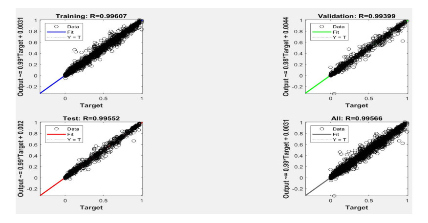
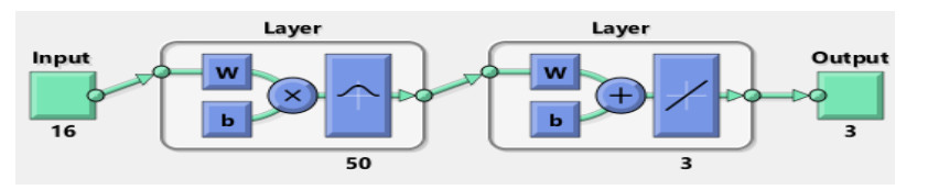
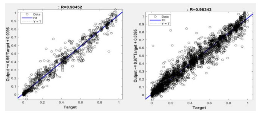
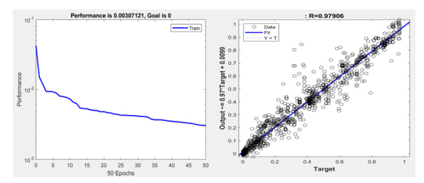
Integrated gas lift system optimization plays an indispensable role in production and economics by maximizing the revenue from a gas lift field. This requires: optimization of gas lift parameters, finding the best tuning of the completion and surface production systems to keep pace with the dynamic reservoir changes along with saving gas quantities and compression costs. Accordingly, a comprehensive study is being carried out to measure the capability of the Artificial Neural Network (ANN) and Machine Learning (ML) in the optimization of gas lift parameters. The results of this study show the power of two different mechanisms of neural network (NN) which are Radial Base Function (RBF) and Back Propagation Function (BPF) to predict the most three important factors of the process: optimal gas injection rate, bottom hole pressure and flow rate and compare the findings with conventional methods. In addition, this work provides 3 functional equations that can be utilized by applying the field data with no artificial intelligence (AI) expertise or software knowledge. This effort provides forth an industrial insight into the role of data-driven computational models for the production recognition scheme, not only to validate the well tests, but also to reduce the uncertainties in production optimization. The work was completed by generating an economic analysis to illustrate the understanding of potential benefits of implementing irregular gas lift mechanisms in the field to stand on both technical and economic aspects of the study.

| [1] |
Farshad FF, Garber JD, Lorde JN (2000) Predicting temperature profiles in producing oil wells using artificial neural networks. Eng Comput 17: 735-754. doi: 10.1108/02644400010340651

|
| [2] |
Tariq Z, Mahmoud M, Abdulraheem A (2019) Core log integration: a hybrid intelligent data-driven solution to improve elastic parameter prediction. Neural Comput Appl 31: 8561-8581. doi: 10.1007/s00521-019-04101-3
|
| [3] |
Mahmoud M (2019) New correlation for the gas deviation factor for high-temperature and high-pressure gas reservoirs using neural networks. Energy Fuels 33: 2426-2436. doi: 10.1021/acs.energyfuels.9b00171
|
| [4] | Olabisi OT, Atubokiki AJ, Babawale O (2019) Artificial neural network for prediction of hydrate formation temperature. Soc Pet Eng. Available from: https://onepetro.org/SPENAIC/proceedings-abstract/19NAIC/2-19NAIC/D023S026R009/219498. |
| [5] | Tariq Z, Abdulraheem A, Khan MR, et al. (2018a) New inflow performance relationship for a horizontal well in a naturally fractured solution gas drive reservoirs using artificial intelligence technique. In: Offshore technology conference Asia. Offshore Technology Conference. |
| [6] |
Khan MR, Tariq Z, Abdulraheem A (2020) Application of artificial intelligence to estimate oil flow rate in gas-lift wells. Nat Resour Res 29: 4017-4029. doi: 10.1007/s11053-020-09675-7
|
| [7] | Zubarev M, Zubarev D (2019) Use of radial basis function networks for efficient well production allocation. SPE Nigeria Annual Int Conf Exhib. Available from: https://onepetro.org/SPENAIC/proceedings-abstract/19NAIC/2-19NAIC/D023S007R002/219944. |
| [8] |
Ekundayo J, Rezaee R (2019) Effect of equation of states on high pressure volumetric measurements of methane-coal sorption isotherms-part 1: Volumes of free space and methane adsorption isotherms. Energy Fuels 33: 1029-1033. doi: 10.1021/acs.energyfuels.8b04016
|
| [9] | Tariq Z, Abdulraheem A, Khan MR, et al. (2018a) New inflow performance relationship for a horizontal well in a naturally fractured solution gas drive reservoirs using artificial intelligence technique. In: Offshore technology conference Asia. |
| [10] |
El-Moniem MAA, El-Banbi AH (2018) Development of an expert system for selection of multiphase flow correlations. J Pet Explor Prod Technol 8: 1473-1485. doi: 10.1007/s13202-018-0442-7
|
| [11] |
Baziar S, Shahripour HB, Tadayoni M, et al. (2018) Prediction of water saturation in a tight gas sandstone reservoir by using four intelligent methods: a comparative study. Neural Comput Appl 30: 1171-1185. doi: 10.1007/s00521-016-2729-2
|
| [12] | Tariq Z (2018) An automated flowing bottom-hole pressure prediction for a vertical well having multiphase flow using computational intelligence techniques. J Pet Explor Prod Technol 354: 463-472. |
| [13] |
Chen W, Di Q, Ye F, et al. (2017) Flowing bottom hole pressure prediction for gas wells based on support vector machine and random samples selection. Int J Hydrogen Energy 42: 18333-18342. doi: 10.1016/j.ijhydene.2017.04.134
|
| [14] |
Bazargan H, Adibifard M (2017) A stochastic well-test analysis on transient pressure data using iterative ensemble Kalman filter. Neural Comput Appl 31: 3227-3243. doi: 10.1007/s00521-017-3264-5
|
| [15] |
Jahed AD, Shoib R, Faizi K, et al. (2017) Developing a hybrid PSO ANN model for estimating the ultimate bearing capacity of rock-socketed piles. Neural Comput Appl 28: 391-405. doi: 10.1007/s00521-015-2072-z
|
| [16] |
Al-Fatlawi O, Hossain MM, Osborne J (2017) Determination of best possible correlation for gas compressibility factor to accurately predict the initial gas reserves in gas-hydrocarbon reservoirs. Int J Hydrogen Energy 42: 25492-25508. doi: 10.1016/j.ijhydene.2017.08.030
|
| [17] |
Shokir EM, Hamed MMB, Ibrahim ESB, et al. (2017) Gas lift optimization using artificial neural network and integrated production modeling. Energy Fuels 31: 9302-9307. doi: 10.1021/acs.energyfuels.7b01690
|


Figures(18) / Tables(7)

Ahmed A. Elgibaly, Mohamed Ghareeb, Said Kamel, Mohamed El-Sayed El-Bassiouny. Prediction of gas-lift performance using neural network analysis[J]. AIMS Energy, 2021, 9(2): 355-378. doi: 10.3934/energy.2021019


 DownLoad: