A possible interpretation of financial markets affected by dark volatility

Richard Pinčák; Alexander Pigazzini; Saeid Jafari; Özge Korkmaz; Cenap Özel; Erik Bartoš; Richard Pinčák; Alexander Pigazzini; Saeid Jafari; Özge Korkmaz; Cenap Özel; Erik Bartoš

doi:10.3934/cam.2023006

Communications in Analysis and Mechanics

2023, Volume 15, Issue 2: 91-110. doi: 10.3934/cam.2023006

Previous Article Next Article

Research article

A possible interpretation of financial markets affected by dark volatility

1.
Institute of Experimental Physics, Slovak Academy of Sciences, Watsonova 47,043 53 Košice, Slovak Republic
2.
Mathematical and Physical Science Foundation, 4200 Slagelse, Denmark
3.
College of Vestsjaelland South, Herrestraede 11, 4200 Slagelse, Denmark
4.
Malatya Turgut Özal University, Department of Management Information Systems, Malatya, Turkey
5.
King Abdulaziz University, Department of Mathematics, 21589 Jeddah, Saudi Arabia
6.
Institute of Physics, Slovak Academy of Sciences, Dúbravská cesta 9,845 11 Bratislava, Slovak Republic

Received: 28 September 2022 Revised: 28 March 2023 Accepted: 30 March 2023 Published: 21 April 2023
53A31, 91G15

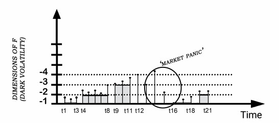
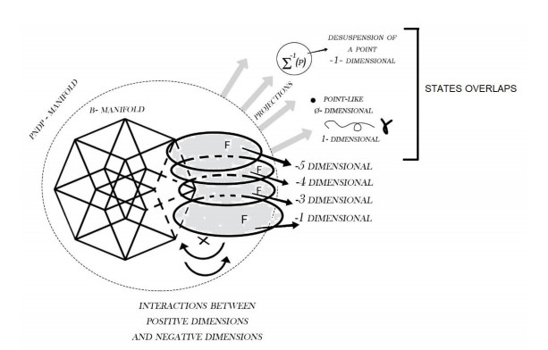
The aim of this paper is to use a special type of Einstein warped product manifolds recently introduced, the so-called PNDP-manifolds, for the differential geometric study, by focusing on some aspects related to dark field in financial market such as the concept of dark volatility. This volatility is not fixed in any relevant economic parameter, a sort of negative dimension, a ghost field, that greatly influences the behavior of real market. Since the PNDP-manifold has a "virtual" dimension, we want to use it in order to show how the Global Market is influenced by dark volatility, and in this regard we also provide an example, by considering the classical exponential models as possible solutions to our approach. We show how dark volatility, combined with specific conditions, leads to the collapse of a forward price.
- dark volatility,
- negative dimension,
- virtual dimension,
- econophysics,
- financial market,
- ghost field
Citation: Richard Pinčák, Alexander Pigazzini, Saeid Jafari, Özge Korkmaz, Cenap Özel, Erik Bartoš. A possible interpretation of financial markets affected by dark volatility[J]. Communications in Analysis and Mechanics, 2023, 15(2): 91-110. doi: 10.3934/cam.2023006

Related Papers:

Abstract

The aim of this paper is to use a special type of Einstein warped product manifolds recently introduced, the so-called PNDP-manifolds, for the differential geometric study, by focusing on some aspects related to dark field in financial market such as the concept of dark volatility. This volatility is not fixed in any relevant economic parameter, a sort of negative dimension, a ghost field, that greatly influences the behavior of real market. Since the PNDP-manifold has a "virtual" dimension, we want to use it in order to show how the Global Market is influenced by dark volatility, and in this regard we also provide an example, by considering the classical exponential models as possible solutions to our approach. We show how dark volatility, combined with specific conditions, leads to the collapse of a forward price.

References

[1]	M. O. Katanaev, T. Klösch, W. Kummer, Global Properties of Warped Solutions in General Relativity, Ann. Phys., 276 (1999), 191–222. https://doi.org/10.1006/aphy.1999.5923 doi: 10.1006/aphy.1999.5923
[2]	C. He, P. Petersen, W. Wylie, Warped product Einstein metrics over spaces with constant scalar curvature, Asian J. Math., 18 (2014), 159–190. https://doi.org/10.4310/AJM.2014.v18.n1.a9 doi: 10.4310/AJM.2014.v18.n1.a9
[3]	X. An, W. W. Y. Wong, Warped product space-times, Class. Quantum Grav., 35 (2018), 025011. https://doi.org/10.1088/1361-6382/aa8af7 doi: 10.1088/1361-6382/aa8af7
[4]	A. Pigazzini, C. Özel, P. Linker, S. Jafari, On a new kind of einstein warped product (POLJ)-manifold, Poincare J. Anal. Appl., 6 (2019), 77–83. https://doi.org/10.46753/pjaa.2019.v06i02.001 doi: 10.46753/pjaa.2019.v06i02.001
[5]	A. Pigazzini, C. Özel, P. Linker, S. Jafari, Corrigendum: On a new kind of Einstein warped product (POLJ)-manifold (PJAA (2019)), Poincare J. Anal. Appl., 7 (2020), 149–150. https://doi.org/10.46753/pjaa.2020.v07i01.012 doi: 10.46753/pjaa.2020.v07i01.012
[6]	R. Pincak, A. Pigazzini, S. Jafari, C. Özel, The "emerging" reality from "hidden" spaces. Universe, 7 (2021), 75. https://doi.org/10.3390/universe7030075 doi: 10.3390/universe7030075
[7]	R. N. Mantegna, H. Eugene Stanley, Introduction to Econophysics: Correlations and Complexity in Finance. Cambridge University Press, 1 edition, 2007.
[8]	S. Farinelli, Geometric arbitrage theory and market dynamics, J. Geom. Mech., 7 (2015), 431–471. https://doi.org/10.3934/jgm.2015.7.431 doi: 10.3934/jgm.2015.7.431
[9]	S. Capozziello, R. Pincak, K. Kanjamapornkul, Anomaly on Superspace of Time Series Data, Z. Naturforsch., 72 (2017), 1077–1091. https://doi.org/10.1515/zna-2017-0274 doi: 10.1515/zna-2017-0274
[10]	R. Pincak, K. Kanjamapornkul, GARCH(1, 1) model of the financial market with the minkowski metric. Z. Naturforsch., 73 (2018), 669–684. https://doi.org/10.1515/zna-2018-0199 doi: 10.1515/zna-2018-0199
[11]	K. Kanjamapornkul, R. Pinčák. Kolmogorov space in time series data, Math. Methods Appl. Sci., 39 (2016), 4463–4483. https://doi.org/10.1002/mma.3875 doi: 10.1002/mma.3875
[12]	A. P. Kirman, G. Teyssière, Long Memory in Economics, Springer Berlin, Heidelberg, 1 edition, 9, 2007. https://doi.org/10.1007/978-3-540-34625-8
[13]	E. Bartoš, R. Pinčák, Identification of market trends with string and D2-brane maps, Phys. A, 479 (2017), 57–70. https://doi.org/10.1016/j.physa.2017.03.014 doi: 10.1016/j.physa.2017.03.014
[14]	K. Kanjamapornkul, R. Pinčák, E. Bartoš. Cohomology theory for financial time series. Phys. A, 546 (2020), 122212. https://doi.org/10.1016/j.physa.2019.122212 doi: 10.1016/j.physa.2019.122212
[15]	K. Kanjamapornkul, R. Pinčák, E. Bartoš, The study of Thai stock market across the 2008 financial crisis. Phys. A, 462 (2016), 117–133. https://doi.org/10.1016/j.physa.2016.06.078 doi: 10.1016/j.physa.2016.06.078
[16]	R. Pincak, D-brane solutions under market panic, Int. J. Geome. Methods Mod. Phys., 15 (2018), 1850099. https://doi.org/10.1142/S0219887818500998 doi: 10.1142/S0219887818500998
[17]	R. Engle, Risk and volatility: Econometric models and financial practice, Am. Econ. Rev., 94 (2004), 405–420. https://doi.org/10.1257/0002828041464597 doi: 10.1257/0002828041464597
[18]	Z. Kostanjčar, S. Begušić, H. E. Stanley, B. Podobnik, Estimating tipping points in feedback-driven financial networks, IEEE J. Sel. Top. Signal Process., 10 (2016), 1040–1052. https://doi.org/10.1109/JSTSP.2016.2593099 doi: 10.1109/JSTSP.2016.2593099
[19]	O. Peters, The ergodicity problem in economics, Nat. Phys., 15 (2019), 1216–1221. https://doi.org/10.1038/s41567-019-0732-0 doi: 10.1038/s41567-019-0732-0
[20]	M. Mangalam, D. G. Kelty-Stephen, Point estimates, simpson's paradox, and nonergodicity in biological sciences, Neurosci. Biobehav. Rev., 125 (2021), 98–107. https://doi.org/10.1016/j.neubiorev.2021.02.017 doi: 10.1016/j.neubiorev.2021.02.017
[21]	A. G. Cherstvy, D. Vinod, E. Aghion, A. V. Chechkin, R. Metzler, Time averaging, ageing and delay analysis of financial time series. New J. Phys., 19 (2017), 063045. https://doi.org/10.1088/1367-2630/aa7199 doi: 10.1088/1367-2630/aa7199
[22]	A. G. Cherstvy, D. Vinod, E. Aghion, I. M. Sokolov, R. Metzler, Scaled geometric brownian motion features sub- or superexponential ensemble-averaged, but linear time-averaged mean-squared displacements. Phys. Rev. E, 103 (2021), 062127. https://doi.org/10.1103/PhysRevE.103.062127 doi: 10.1103/PhysRevE.103.062127
[23]	D. Joyce, Kuranishi spaces and Symplectic Geometry. Volume Ⅱ. Differential Geometry of (m-)Kuranishi spaces. The Mathematical Institute, Oxford, UK, 2017.
[24]	U. C. De, S. Shenawy, B. Ünal, Sequential warped products: Curvature and conformal vector fields, Filomat, 33 (2019), 4071–4083. https://doi.org/10.2298/FIL1913071D doi: 10.2298/FIL1913071D
[25]	S. Pahan, B. Pal, On einstein sequential warped product spaces, J. Math. Phys. Anal. Geom., 15 (2019), 379–394. https://doi.org/10.15407/mag15.03.379 doi: 10.15407/mag15.03.379
[26]	M. Atçeken, S. Keleş, On the product riemannian manifolds, Differ. Geom. Dyn. Syst., 5 (2003), 1–8.
[27]	F. Black, The pricing of commodity contracts, J. Financ. Econ., 3 (1976), 167–179. https://doi.org/10.1016/0304-405X(76)90024-6 doi: 10.1016/0304-405X(76)90024-6
[28]	F. Black, M. Scholes, The pricing of options and corporate liabilities, J. Political Econ., 81 (1973), 637–657. https://doi.org/10.1086/260062 doi: 10.1086/260062
[29]	J. Bertoin, Lévy Processes, volume 121 of Cambridge Tracts in Mathematics. Cambridge University Press, Cambridge, 1998.
[30]	P. Jäckel, py_vollib python library package, 2014. Available from: http://vollib.org/documentation/python/1.0.2/#.
[31]	Yahoo! Finance historical prices, 2022. Available from: https://finance.yahoo.com.
[32]	P. Hsu, Brownian Motion and Riemannian Geometry, Contemp. Math., 73 (1988), 95–104. http://dx.doi.org/10.1090/conm/073/954633 doi: 10.1090/conm/073/954633
[33]	E. P. Hsu, Stochastic Analysis on Manifolds, volume 38. American Mathematical Society, 2002.
[34]	H. Zhang, W. Tang, P. Zhao, Asian option on Riemannian manifolds, Int. J. Bus. Mark. Manage., 5 (2020), 67–80.

Reader Comments

Your name:*

Email:*
© 2023 the Author(s), licensee AIMS Press. This is an open access article distributed under the terms of the Creative Commons Attribution License (http://creativecommons.org/licenses/by/4.0)