The association of self-reported physical activity on human sensory long-term potentiation

Damien Moore; Paul D Loprinzi; Damien Moore; Paul D Loprinzi

doi:10.3934/Neuroscience.2021023

AIMS Neuroscience

2021, Volume 8, Issue 3: 435-447. doi: 10.3934/Neuroscience.2021023

Previous Article Next Article

Research article Special Issues

The association of self-reported physical activity on human sensory long-term potentiation

Damien Moore ,
Paul D Loprinzi ^,

Exercise & Memory Laboratory, Department of Health, Exercise Science and Recreation Management, The University of Mississippi, University, MS 38677, USA

Received: 17 April 2021 Accepted: 20 May 2021 Published: 24 May 2021

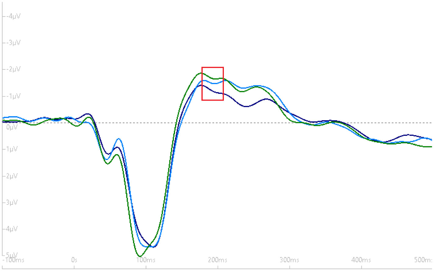
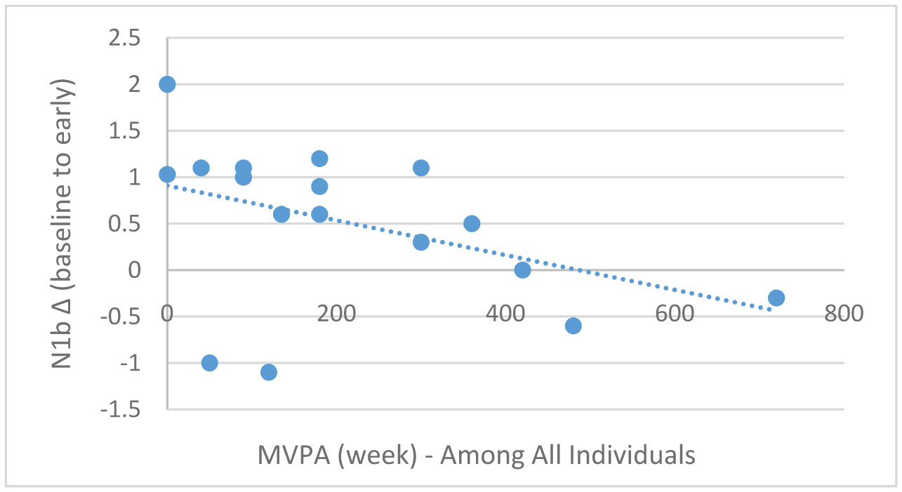
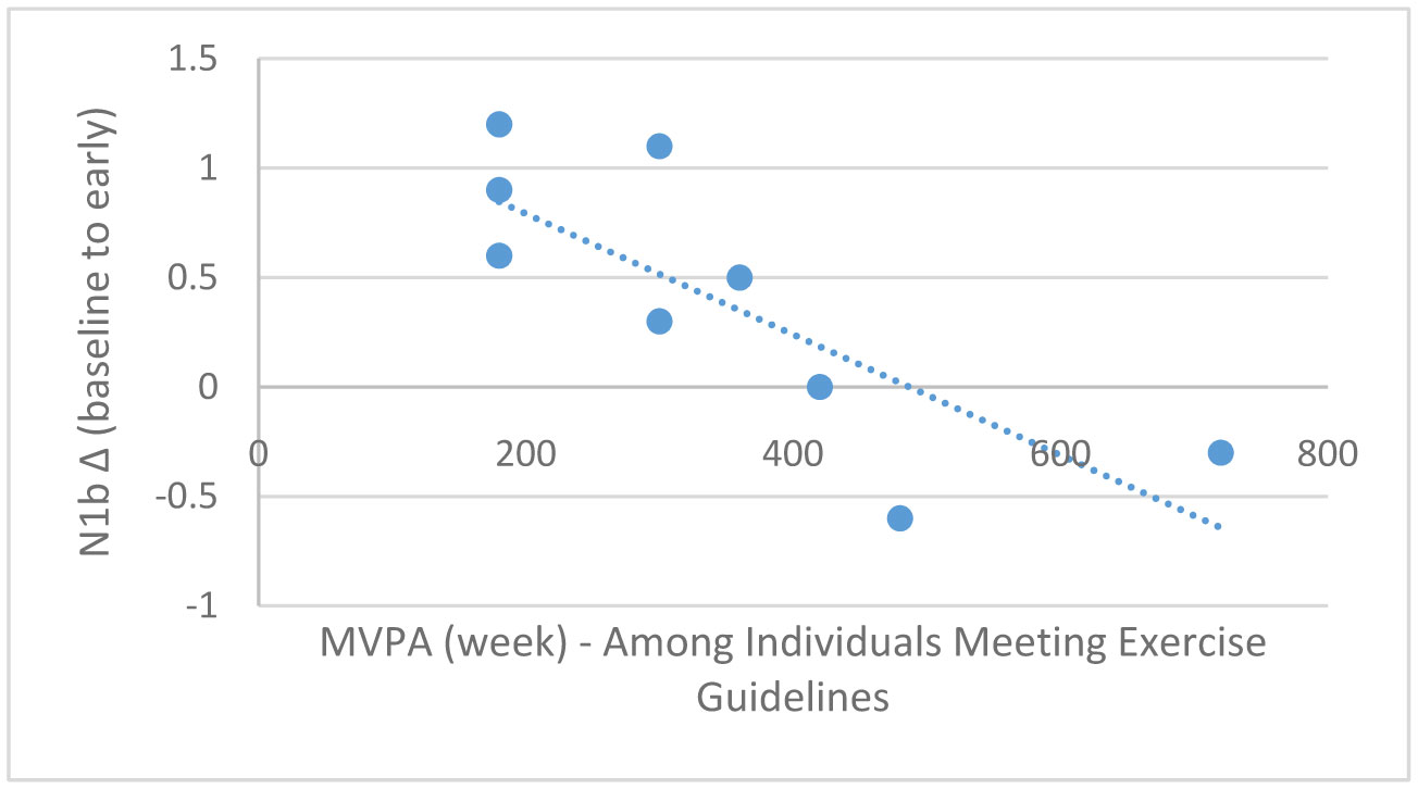
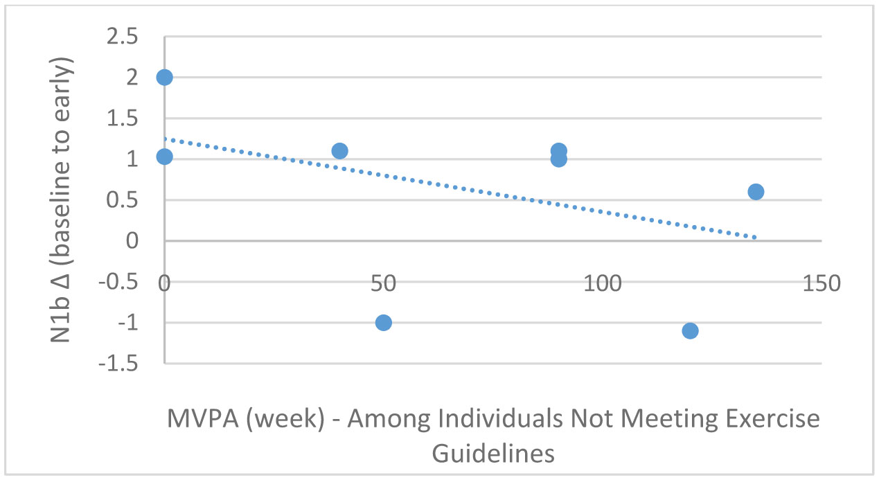
Exercise has been shown to enhance synaptic plasticity, therefore, potentially affecting memory. While the mechanism(s) responsible for this relationship have been explored in animal models, current research suggests that exercise may possess the ability to induce synaptic long-term potentiation (LTP). Most of the LTP mechanistic work has been conducted in animal models using invasive procedures. For that reason, the purpose of the present experiment was to investigate whether self-reported exercise is related to human sensory LTP-like responses. Nineteen participants (M_AGE = 24 years; 52.6% male) completed the study. Long-term potentiation-like responses were measured by incorporating a non-invasive method that assess the change in potentiation of the N1b component produced from the visual stimulus paradigm presented bilaterally in the visual field. Results demonstrated that those with higher levels of moderate-to-vigorous physical activity (MVPA) had a greater N1b change from baseline to the early time period assessment, r = −0.43, p = 0.06. Our findings provide some suggestive evidence of an association between self-reported MVPA and LTP-like responses. Additional work is needed to support that the potentiation of the human sensory N1b component in the observed study is due to the exercise-induced synaptic changes similar to that detailed in prior animal research.
- electroencephalogram,
- exercise,
- memory,
- long-term potentiation,
- synaptic plasticity
Citation: Damien Moore, Paul D Loprinzi. The association of self-reported physical activity on human sensory long-term potentiation[J]. AIMS Neuroscience, 2021, 8(3): 435-447. doi: 10.3934/Neuroscience.2021023

Related Papers:

Abstract

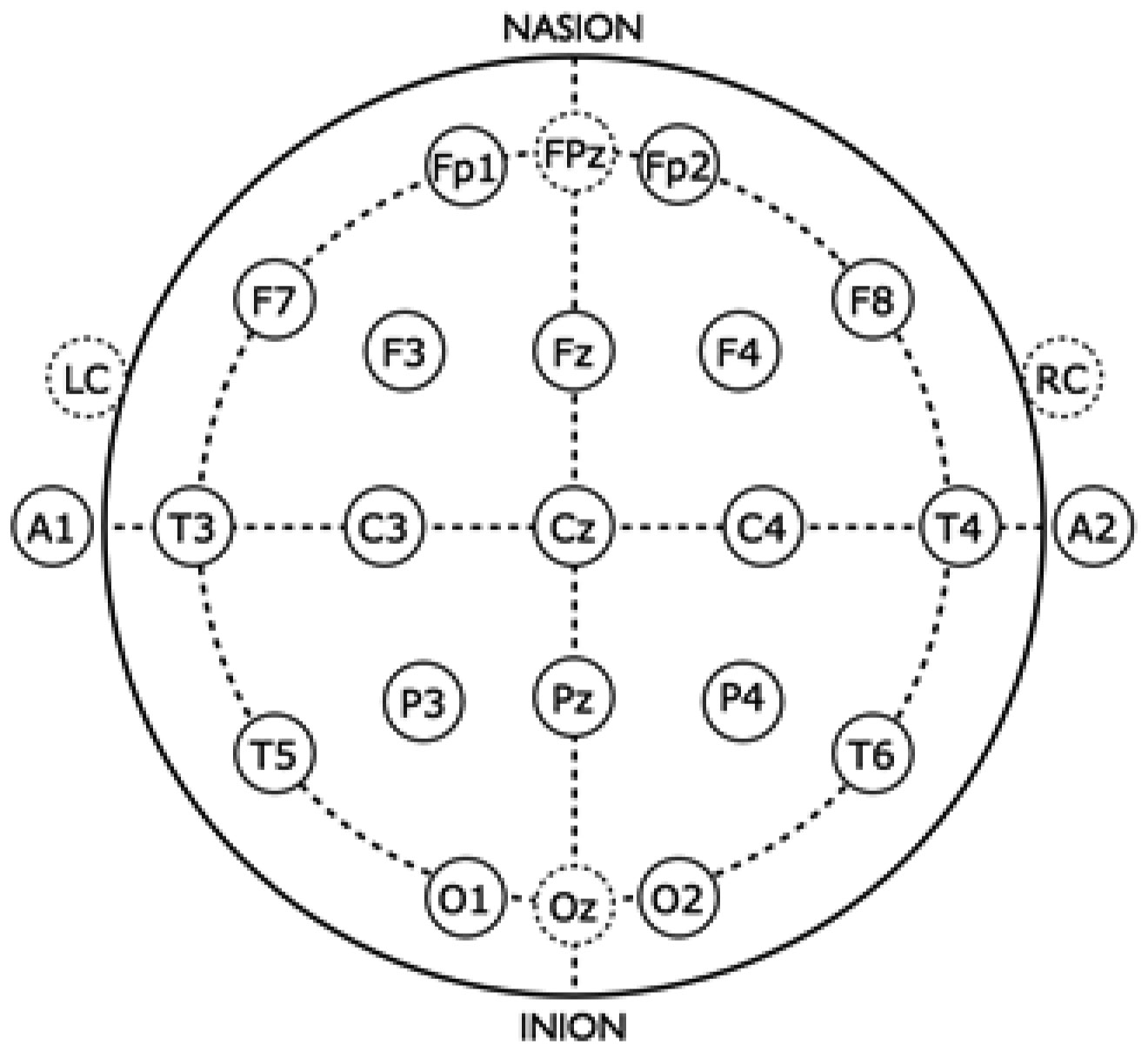
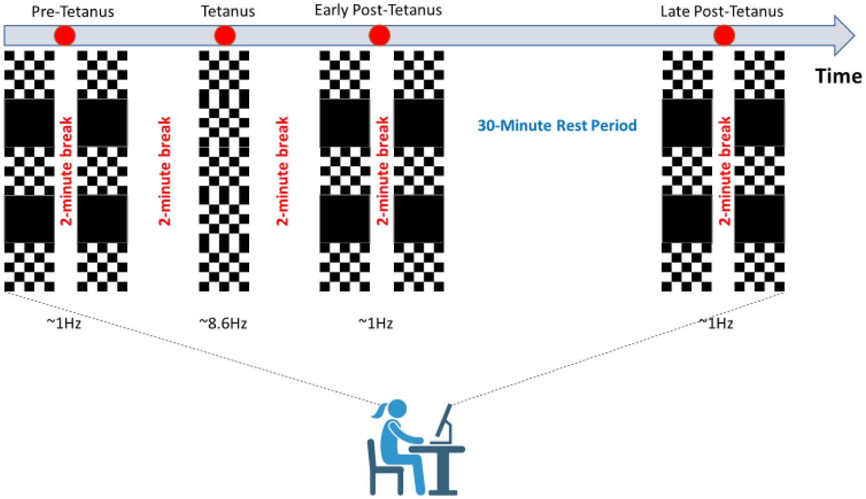
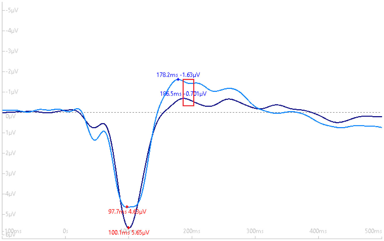
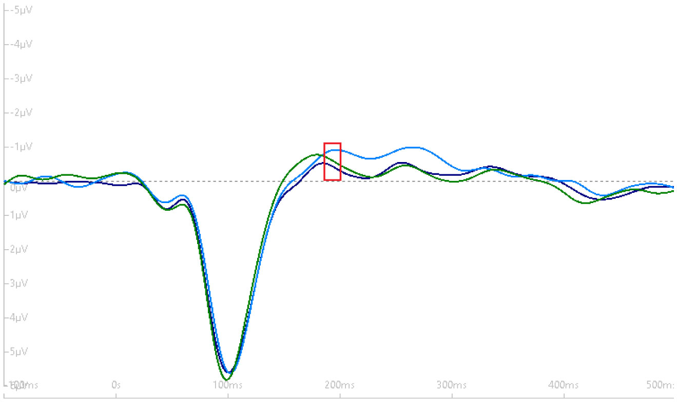
Exercise has been shown to enhance synaptic plasticity, therefore, potentially affecting memory. While the mechanism(s) responsible for this relationship have been explored in animal models, current research suggests that exercise may possess the ability to induce synaptic long-term potentiation (LTP). Most of the LTP mechanistic work has been conducted in animal models using invasive procedures. For that reason, the purpose of the present experiment was to investigate whether self-reported exercise is related to human sensory LTP-like responses. Nineteen participants (M_AGE = 24 years; 52.6% male) completed the study. Long-term potentiation-like responses were measured by incorporating a non-invasive method that assess the change in potentiation of the N1b component produced from the visual stimulus paradigm presented bilaterally in the visual field. Results demonstrated that those with higher levels of moderate-to-vigorous physical activity (MVPA) had a greater N1b change from baseline to the early time period assessment, r = −0.43, p = 0.06. Our findings provide some suggestive evidence of an association between self-reported MVPA and LTP-like responses. Additional work is needed to support that the potentiation of the human sensory N1b component in the observed study is due to the exercise-induced synaptic changes similar to that detailed in prior animal research.

¹ NMDA receptor saturation is a period in which all receptors are successfully occupied with the neurotransmitter glutamate.

² NMDA receptor longevity reflects the length of time the ligand is bound to the receptor(s) before the ligand disassociates, reducing the activity/function of the receptors.

Conflict of interest

The authors declare no conflict of interest.

References

[1]	Gomez-Pinilla F, Hillman C (2013) The influence of exercise on cognitive abilities. Compr Physiol 3: 403-428.
[2]	Loprinzi P (2019) The Effects of Exercise on Long-Term Potentiation: A Candidate Mechanism of the Exercise-Memory Relationship. OBM Neurobiol 3: 1. doi: 10.21926/obm.neurobiol.1902026
[3]	Roig M, Nordbrandt S, Geertsen SS, et al. (2013) The effects of cardiovascular exercise on human memory: A review with meta-analysis. Neurosci Biobehav Rev 37: 1645-1666. doi: 10.1016/j.neubiorev.2013.06.012
[4]	Cooke SF, Bliss TV (2006) Plasticity in the human central nervous system. Brain 129: 1659-1673. doi: 10.1093/brain/awl082
[5]	Clapp WC, Eckert MJ, Teyler TJ, et al. (2006) Rapid visual stimulation induces N-methyl-D-aspartate receptor-dependent sensory long-term potentiation in the rat cortex. Neuroreport 17: 511-515. doi: 10.1097/01.wnr.0000209004.63352.10
[6]	Manabe T (2017) NMDA receptor-independent long-term potentiation in hippocampal interneurons. J Physiol 595: 3263-3264. doi: 10.1113/JP274093
[7]	Bliss TV, Lomo T (1973) Long-lasting potentiation of synaptic transmission in the dentate area of the anaesthetized rabbit following stimulation of the perforant path. J Physiol 232: 331-356. doi: 10.1113/jphysiol.1973.sp010273
[8]	Bliss TVP, Cooke SF (2011) Long-term potentiation and long-term depression: a clinical perspective. Clinics 66: 3-17. doi: 10.1590/S1807-59322011001300002
[9]	Nicoll RA (2017) A Brief History of Long-Term Potentiation. Neuron 93: 281-290. doi: 10.1016/j.neuron.2016.12.015
[10]	Aberg KC, Herzog MH (2012) About similar characteristics of visual perceptual learning and LTP. Vision Res 61: 100-106. doi: 10.1016/j.visres.2011.12.013
[11]	Radahmadi M, Hosseini N, Alaei H (2016) Effect of exercise, exercise withdrawal, and continued regular exercise on excitability and long-term potentiation in the dentate gyrus of hippocampus. Brain Res 1653: 8-13. doi: 10.1016/j.brainres.2016.09.045
[12]	Van Dongen EV, Kersten IHP, Wagner IC, et al. (2016) Physical Exercise Performed Four Hours after Learning Improves Memory Retention and Increases Hippocampal Pattern Similarity during Retrieval. Curr Biol 26: 1722-1727. doi: 10.1016/j.cub.2016.04.071
[13]	Mellow ML, Goldsworthy MR, Coussens S, et al. (2020) Acute aerobic exercise and neuroplasticity of the motor cortex: A systematic review. J Sci Med Sport 23: 408-414. doi: 10.1016/j.jsams.2019.10.015
[14]	Singh AM, Staines WR (2015) The effects of acute aerobic exercise on the primary motor cortex. J Mot Behav 47: 328-339. doi: 10.1080/00222895.2014.983450
[15]	Ross RM, McNair NA, Fairhall SL, et al. (2008) Induction of orientation-specific LTP-like changes in human visual evoked potentials by rapid sensory stimulation. Brain Res Bull 76: 97-101. doi: 10.1016/j.brainresbull.2008.01.021
[16]	Smallwood N, Spriggs MJ, Thompson CS, et al. (2015) Influence of Physical Activity on Human Sensory Long-Term Potentiation. J Int Neuropsychol Soc 21: 831-840. doi: 10.1017/S1355617715001095
[17]	Teyler TJ, Hamm JP, Clapp WC, et al. (2005) Long-term potentiation of human visual evoked responses. Eur J Neurosci 21: 2045-2050. doi: 10.1111/j.1460-9568.2005.04007.x
[18]	McNair NA, Clapp WC, Hamm JP, et al. (2006) Spatial frequency-specific potentiation of human visual-evoked potentials. Neuroreport 17: 739-741. doi: 10.1097/01.wnr.0000215775.53732.9f
[19]	Clapp WC, Hamm JP, Kirk IJ, et al. (2012) Translating long-term potentiation from animals to humans: a novel method for noninvasive assessment of cortical plasticity. Biol Psychiatry 71: 496-502. doi: 10.1016/j.biopsych.2011.08.021
[20]	Spriggs MJ, Thompson CS, Moreau D, et al. (2019) Human Sensory LTP Predicts Memory Performance and Is Modulated by the BDNF Val⁶⁶Met Polymorphism. Front Hum Neurosci 13: 22. doi: 10.3389/fnhum.2019.00022
[21]	Heynen AJ, Bear MF (2001) Long-term potentiation of thalamocortical transmission in the adult visual cortex in vivo. J Neurosci 21: 9801-9813. doi: 10.1523/JNEUROSCI.21-24-09801.2001
[22]	Moore D, Ikuta T, Loprinzi PD (2020) The Effects of Human Visual Sensory Stimuli on N1b Amplitude: An EEG Study. J Clin Med 9: 2837. doi: 10.3390/jcm9092837
[23]	Ball TJ, Joy EA, Gren LH, et al. (2016) Predictive Validity of an Adult Physical Activity “Vital Sign” Recorded in Electronic Health Records. J Phys Act Health 13: 403-408. doi: 10.1123/jpah.2015-0210
[24]	Ball TJ, Joy EA, Gren LH, et al. (2016) Concurrent Validity of a Self-Reported Physical Activity “Vital Sign” Questionnaire With Adult Primary Care Patients. Prev Chronic Dis 13: E16.
[25]	Ferree TC, Luu P, Russell GS, et al. (2001) Scalp electrode impedance, infection risk, and EEG data quality. Clin Neurophysiol 112: 536-544. doi: 10.1016/S1388-2457(00)00533-2
[26]	Bull FC, Al-Ansari SS, Biddle S, et al. (2020) World Health Organization 2020 guidelines on physical activity and sedentary behaviour. Br J Sports Med 54: 1451-1462. doi: 10.1136/bjsports-2020-102955
[27]	Li YT, Liu BH, Chou XL, et al. (2015) Synaptic Basis for Differential Orientation Selectivity between Complex and Simple Cells in Mouse Visual Cortex. J Neurosci 35: 11081-11093. doi: 10.1523/JNEUROSCI.5246-14.2015
[28]	Sato H, Katsuyama N, Tamura H, et al. (1996) Mechanisms underlying orientation selectivity of neurons in the primary visual cortex of the macaque. J Physiol 494: 757-771. doi: 10.1113/jphysiol.1996.sp021530
[29]	Pang PT, Nagappan G, Guo W, et al. (2016) Extracellular and intracellular cleavages of proBDNF required at two distinct stages of late-phase LTP. NPJ Sci Learn 1: 16003. doi: 10.1038/npjscilearn.2016.3
[30]	Gomez-Pinilla F, Vaynman S, Ying Z (2008) Brain-derived neurotrophic factor functions as a metabotrophin to mediate the effects of exercise on cognition. Eur J Neurosci 28: 2278-2287. doi: 10.1111/j.1460-9568.2008.06524.x
[31]	Loprinzi PD, Moore D, Loenneke JP (2020) Does Aerobic and Resistance Exercise Influence Episodic Memory through Unique Mechanisms? Brain Sci 10: 913. doi: 10.3390/brainsci10120913
[32]	Dunsky A, Abu-Rukun M, Tsuk S, et al. (2017) The effects of a resistance vs. an aerobic single session on attention and executive functioning in adults. PloS One 12: e0176092. doi: 10.1371/journal.pone.0176092
[33]	Liu-Ambrose T, Donaldson MG (2009) Exercise and cognition in older adults: is there a role for resistance training programmes? Br J Sports Med 43: 25-27. doi: 10.1136/bjsm.2008.055616

Reader Comments

Your name:*

Email:*
© 2021 the Author(s), licensee AIMS Press. This is an open access article distributed under the terms of the Creative Commons Attribution License (http://creativecommons.org/licenses/by/4.0)