A High-Order Symmetric Interior Penalty Discontinuous Galerkin Scheme
to Simulate Vortex Dominated Incompressible Fluid Flow

Song Lunji; Song Lunji

doi:10.3934/Math.2016.1.43

AIMS Mathematics

2016, Volume 1, Issue 1: 43-63. doi: 10.3934/Math.2016.1.43

Previous Article Next Article

Research article

A High-Order Symmetric Interior Penalty Discontinuous Galerkin Scheme to Simulate Vortex Dominated Incompressible Fluid Flow

Song Lunji ^{1,2
,
,}

1.
School of Mathematics and Statistics, Lanzhou University, Lanzhou, 730000, China
2.
Department of Mathematics, The University of Alabama, Tuscaloosa, AL 35487, USA
3.
Department of Aerospace Engineering and Mechanics, The University of Alabama, Tuscaloosa, AL 35487, USA

Received: 16 April 2016 Accepted: 25 April 2016 Published: 27 April 2016

A high-order Symmetric Interior Penalty discontinuous Galerkin (SIPG) method has been used for solving the incompressible Navier-Stokes equation. We apply the temporal splitting scheme in time and the SIPG discretization in space with the local Lax-Friedrichs flux for the discretization of nonlinear terms. A fully discrete semi-implicit splitting scheme has been presented and high-order discontinuous Galerkin (DG) finite elements are available. Under a constraint of the CFL condition, two benchmark problems in 2D are investigated: one is a lid-driven cavity flow to verify the high-order discontinuous Galerkin method is accurate and robust; the other is a flow past a circular cylinder, for which we mainly check the Strouhal numbers with the von Kármán vortex street, and also simulate the boundary layers with walls and corresponding dynamical behavior with Neumann conditions on the top and bottom boundaries, respectively. We predict the Strouhal number for the range of Reynolds number 50 ≤ Re ≤ 400, making a comparison between the predicted values by our numerical method and the referenced values from physical experiments.
- Navier-Stokes equations,
- von K´arm´an vortex street,
- discontinuous Galerkin method,
- interior penalty
Citation: Song Lunji. A High-Order Symmetric Interior Penalty Discontinuous Galerkin Schemeto Simulate Vortex Dominated Incompressible Fluid Flow[J]. AIMS Mathematics, 2016, 1(1): 43-63. doi: 10.3934/Math.2016.1.43

Related Papers:

Abstract

A high-order Symmetric Interior Penalty discontinuous Galerkin (SIPG) method has been used for solving the incompressible Navier-Stokes equation. We apply the temporal splitting scheme in time and the SIPG discretization in space with the local Lax-Friedrichs flux for the discretization of nonlinear terms. A fully discrete semi-implicit splitting scheme has been presented and high-order discontinuous Galerkin (DG) finite elements are available. Under a constraint of the CFL condition, two benchmark problems in 2D are investigated: one is a lid-driven cavity flow to verify the high-order discontinuous Galerkin method is accurate and robust; the other is a flow past a circular cylinder, for which we mainly check the Strouhal numbers with the von Kármán vortex street, and also simulate the boundary layers with walls and corresponding dynamical behavior with Neumann conditions on the top and bottom boundaries, respectively. We predict the Strouhal number for the range of Reynolds number 50 ≤ Re ≤ 400, making a comparison between the predicted values by our numerical method and the referenced values from physical experiments.

References

[1]	J. B. Barlow, W. H. Rae, and A. Pope (1999) Low-Speed Wind Tunnel Testing, John Wiley.
[2]	A. J. Chorin (1969) On the convergence of discrete approximations to the Navier-Stokes equations, Math. Comp., 23.
[3]	M. Drela (2014) Flight Vehicle Aerodynamics.MIT Press, Boston .
[4]	Y. Epshteyn, B. Rivi`ere (2007) Estimation of penalty parameters for symmetric interior penalty Galerkin methods,.J. Comput. Appl. Math., 206 .
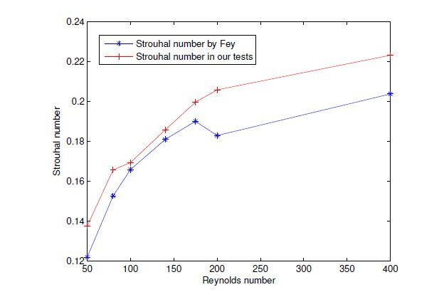
[5]	U. Fey, M. K¨onig, and H. Eckelmann (1998) A new Strouhal-Reynolds-number relationship for the circular cylinder in the range 47 ≤ Re ≤ 2 × 105,.Physics of Fluids 1547-1549.
[6]	U.Ghia, K. N. Ghia, C. T. Shin (1982) High-Re solutions for incompressible flow using the Navier-Stokes equations and a multigrid method..J. Comput. Phys., 48: 387-411.
[7]	V. Girault, B. Rivi`ere, and M. F. Wheeler (2005) A splitting method using discontinuous Galerkin for the transient incompressible Navier-Stokes equations,.ESAIM: Mathematical Modelling and Numerical Analysis, 39: 1115-1147.
[8]	V. Girault, B. Rivi`ere, and M. F. (2005) Wheeler, A discontinuous Galerkin method with non-overlapping domain decomposition for the Stokes and Navier-Stokes problems,.Math. Comp 53-84.
[9]	O. Goyon (1996) High-Reynolds number solutions of Navier-Stokes equations using incremental unknowns,.Comput. Method. Appl. M.130 319-335.
[10]	J. S. Hesthaven (1998) From electrostatics to almost optimal nodal sets for polynomial interpolation in a simplex,.SIAM J. Numer. Anal. 35: 655-676.
[11]	J. S. Hesthaven, C. H. Teng (2000) Stable spectral methods on tetrahedral elements, SIAM.J. Sci. Comput., 2352-2380.
[12]	S. F Hoerner (1965) Fluid-Dynamic Drag, Hoerner Fluid Dynamics.Bakersfield .
[13]	G. Karniadakis, S. J. Sherwin (2005) Spectral/hp element methods for CFD, Oxford University Press.New York .
[14]	S. Kaya, B. Rivi`ere (2005) A discontinuous subgrid eddy viscosity method for the time-dependent Navier-Stokes equations, SIAM J.Numer. Anal 43: 1572-1595.
[15]	B. Rivi`ere, M. F. Wheeler, and V. Girault (1999) Improved energy estimates for interior penalty, constrained and discontinuous Galerkin methods for elliptic problems..Part I, Comput. Geosci., 337-360.
[16]	M. Sch¨afer, S. Turek (1996) The benchmark problem ‘flow around a cylinder’, In Flow Simulation with High-Performance Computers II, Hirschel, E.H.(ed.). Notes on Numerical Fluid Mechanics, vol. 52.Vieweg, Braunschweig, 547-566.
[17]	J. Shen (1991) Hopf bifurcation of the unsteady regularized driven cavity flow,.J. Comput. Phys 95: 228-245.
[18]	J. Shen (1996) On error estimates of the projection methods for the Navier-Stokes equations: Secondorder schemes,.Math. Comp 65: 1039-1065.
[19]	L. Song, Z. Zhang (2015) Polynomial preserving recovery of an over-penalized symmetric interior penalty Galerkin method for elliptic problems,.Discrete Contin. Dyn. Syst. – Ser. B 20: 1405-1426.
[20]	L. Song, Z. Zhang (2015) Superconvergence property of an over-penalized discontinuous Galerkin finite element gradient recovery method,.J. Comput. Phys 299: 1004-1020.
[21]	R. Temam (2001) Navier-Stokes Equations: Theory and Numerical Analysis, AMS Chelsea publishing.Providence .
[22]	R. Temam (1995) Navier-Stokes Equations and Nonlinear Functional Analysis, Volume 66 of CBMSNSF Regional Conference Series in Applied Mathematics.SIAM, Philadelphia, second edition .
[23]	M. F. Wheeler (1978) An elliptic collocation-finite element method with interior penalties,.SIAM J. Numer. Anal., 15: 152-161.

Reader Comments

Your name:*

Email:*
© 2016 the Author(s), licensee AIMS Press. This is an open access article distributed under the terms of the Creative Commons Attribution License (http://creativecommons.org/licenses/by/4.0)