Deep learning-based object detection models perform well under daytime conditions but face significant challenges at night, primarily because they are predominantly trained on daytime images. Additionally, training with nighttime images presents another challenge: Even human annotators struggle to accurately label objects in low-light conditions. This issue is particularly pronounced in transportation applications, such as detecting vehicles and other objects of interest on rural roads at night, where street lighting is often absent, and headlights may introduce undesirable glare. In this study, we addressed these challenges by introducing a novel framework for labeling-free data augmentation, leveraging synthetic data generated by the Car Learning to Act (CARLA) simulator for day-to-night image style transfer. Specifically, the framework incorporated the efficient attention Generative Adversarial Network for realistic day-to-night style transfer and used CARLA-generated synthetic nighttime images to help the model learn the vehicle headlight effect. To evaluate the efficacy of the proposed framework, we fine-tuned the state-of-the-art object detection model with an augmented dataset curated for rural nighttime environments, achieving significant improvements in nighttime vehicle detection. This novel approach was simple yet effective, offering a scalable solution to enhance deep learning-based detection systems in low-visibility environments and extended the applicability of object detection models to broader real-world contexts.
Citation: Yunxiang Yang, Hao Zhen, Yongcan Huang, Jidong J. Yang. Enhancing nighttime vehicle detection with day-to-night style transfer and labeling-free augmentation[J]. Applied Computing and Intelligence, 2025, 5(1): 14-28. doi: 10.3934/aci.2025002
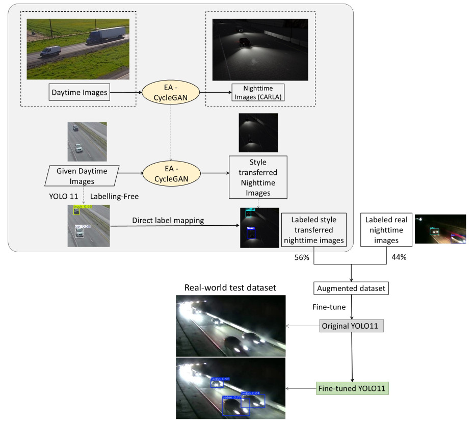
Deep learning-based object detection models perform well under daytime conditions but face significant challenges at night, primarily because they are predominantly trained on daytime images. Additionally, training with nighttime images presents another challenge: Even human annotators struggle to accurately label objects in low-light conditions. This issue is particularly pronounced in transportation applications, such as detecting vehicles and other objects of interest on rural roads at night, where street lighting is often absent, and headlights may introduce undesirable glare. In this study, we addressed these challenges by introducing a novel framework for labeling-free data augmentation, leveraging synthetic data generated by the Car Learning to Act (CARLA) simulator for day-to-night image style transfer. Specifically, the framework incorporated the efficient attention Generative Adversarial Network for realistic day-to-night style transfer and used CARLA-generated synthetic nighttime images to help the model learn the vehicle headlight effect. To evaluate the efficacy of the proposed framework, we fine-tuned the state-of-the-art object detection model with an augmented dataset curated for rural nighttime environments, achieving significant improvements in nighttime vehicle detection. This novel approach was simple yet effective, offering a scalable solution to enhance deep learning-based detection systems in low-visibility environments and extended the applicability of object detection models to broader real-world contexts.

| [1] | National Highway Traffic Safety Administration, Daytime and nighttime seat belt use by fatally injured passenger vehicle occupants, U.S. Department of Transportation, 2010. Available from: https://www.nhtsa.gov/sites/nhtsa.gov/files/documents/811281.pdf. |
| [2] | National Highway Traffic Safety Administration, Report to congress: nighttime glare and driving performance, U.S. Department of Transportation, 2007. Available from: https://www.nhtsa.gov/sites/nhtsa.gov/files/glare_congressional_report.pdf. |
| [3] |
U. Mittal, P. Chawla, R. Tiwari, Ensemblenet: a hybrid approach for vehicle detection and estimation of traffic density based on faster r-cnn and yolo models, Neural Comput. Applic., 35 (2023), 4755–4774. https://doi.org/10.1007/s00521-022-07940-9 doi: 10.1007/s00521-022-07940-9

|
| [4] |
M. Bie, Y. Liu, G. Li, J. Hong, J. Li, Real-time vehicle detection algorithm based on a lightweight you-only-look-once (yolov5n-l) approach, Expert Syst. Appl., 213 (2023), 119108. https://doi.org/10.1016/j.eswa.2022.119108 doi: 10.1016/j.eswa.2022.119108
|
| [5] | S. Huang, C. Lin, S. Chen, Y. Wu, P. Hsu, S. Lai, Auggan: cross domain adaptation with gan-based data augmentation, Proceedings of the European Conference on Computer Vision (ECCV), 2018,718–731. |
| [6] |
G. Bang, J. Lee, Y. Endo, T. Nishimori, K. Nakao, S. Kamijo, Semantic and geometric-aware day-to-night image translation network, Sensors, 24 (2024), 1339. https://doi.org/10.3390/s24041339 doi: 10.3390/s24041339
|
| [7] |
X. Shao, C. Wei, Y. Shen, Z. Wang, Feature enhancement based on cyclegan for nighttime vehicle detection, IEEE Access, 9 (2020), 849–859. https://doi.org/10.1109/ACCESS.2020.3046498 doi: 10.1109/ACCESS.2020.3046498
|
| [8] | J. Zhu, T. Park, P. Isola, A. Efros, Unpaired image-to-image translation using cycle-consistent adversarial networks, Proceedings of the IEEE International Conference on Computer Vision (ICCV), 2017, 2223–2232. |
| [9] |
H. Xu, S. Lai, X. Li, Y. Yang, Cross-domain car detection model with integrated convolutional block attention mechanism, Image Vision Comput., 140 (2023), 104834. https://doi.org/10.1016/j.imavis.2023.104834 doi: 10.1016/j.imavis.2023.104834
|
| [10] |
L. Fu, H. Yu, F. Xu, J. Li, Q. Guo, S. Wang, Let there be light: improved traffic surveillance via detail preserving night-to-day transfer, IEEE Trans. Circ. Syst. Vid., 32 (2022), 8217–8226. https://doi.org/10.1109/TCSVT.2021.3081999 doi: 10.1109/TCSVT.2021.3081999
|
| [11] |
F. Guo, J. Liu, Q. Xie, H. Chang, Improved nighttime traffic detection using day-to-night image transfer, Transport. Res. Rec., 2677 (2023), 711–721. https://doi.org/10.1177/03611981231166686 doi: 10.1177/03611981231166686
|
| [12] | B. Kawar, S. Zada, O. Lang, O. Tov, H. Chang, T. Dekel, et al., Imagic: text-based real image editing with diffusion models, Proceedings of the IEEE/CVF Conference on Computer Vision and Pattern Recognition (CVPR), 2023, 6007–6017. |
| [13] |
Q. Zou, H. Ling, S. Luo, Y. Huang, M. Tian, Robust nighttime vehicle detection by tracking and grouping headlights, IEEE Trans. Intell. Transp., 16 (2015), 2838–2849. https://doi.org/10.1109/TITS.2015.2425229 doi: 10.1109/TITS.2015.2425229
|
| [14] |
S. Parvin, L. Rozario, M. Islam, Vision-based on-road nighttime vehicle detection and tracking using taillight and headlight features, Journal of Computer and Communications, 9 (2021), 107619. https://doi.org/10.4236/jcc.2021.93003 doi: 10.4236/jcc.2021.93003
|
| [15] | A. Dosovitskiy, G. Ros, F. Codevilla, A. Lopez, V. Koltun, Carla: an open urban driving simulator, Proceedings of the 1st Annual Conference on Robot Learning, 2017, 1–16. |
| [16] | R. Khanam, M. Hussain, YOLOv11: an overview of the key architectural enhancements, arXiv: 2410.17725. https://doi.org/10.48550/arXiv.2410.17725 |
| [17] |
S. Malik, M. Khan, H. El-Sayed, Carla: car learning to act—an inside out, Procedia Computer Science, 198 (2022), 742–749. https://doi.org/10.1016/j.procs.2021.12.316 doi: 10.1016/j.procs.2021.12.316
|
| [18] | J. Zhu, T. Park, T. Wang, Efficient-attention-GAN: unsupervised image-to-image translation with shared efficient attention mechanism, GitHub, Inc., 2023. Available from: https://github.com/jccb15/efficient-attention-GAN. |
| [19] | X. Mao, Q. Li, H. Xie, R. Lau, Z. Wang, S. Smolley, Least squares generative adversarial networks, Proceedings of the IEEE International Conference on Computer Vision (ICCV), 2017, 2794–2802. |
| [20] | Y. Taigman, A. Polyak, L. Wolf, Unsupervised cross-domain image generation, arXiv: 1611.02200. https://doi.org/10.48550/arXiv.1611.02200 |
| [21] | T. Lin, M. Maire, S. Belongie, J. Hays, P. Perona, D. Ramanan, et al., Microsoft coco: common objects in context, In: Computer vision—ECCV 2014, Cham: Springer, 2014,740–755. https://doi.org/10.1007/978-3-319-10602-1_48 |
| [22] | K. You, M. Long, J. Wang, M. Jordan, How does learning rate decay help modern neural networks? arXiv: 1908.01878. https://doi.org/10.48550/arXiv.1908.01878 |


Figures(8) / Tables(3)
Yunxiang Yang, Hao Zhen, Yongcan Huang, Jidong J. Yang. Enhancing nighttime vehicle detection with day-to-night style transfer and labeling-free augmentation[J]. Applied Computing and Intelligence, 2025, 5(1): 14-28. doi: 10.3934/aci.2025002


 DownLoad: