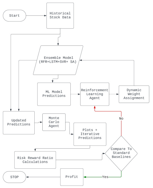
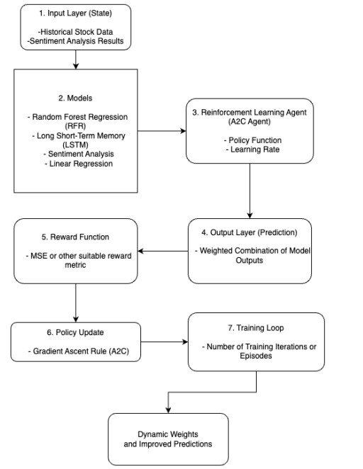
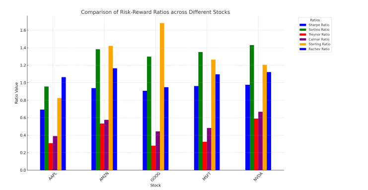
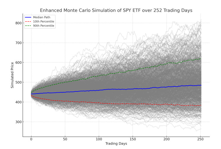
This paper presents a novel integration of Machine Learning (ML) models with Monte Carlo simulations to enhance financial forecasting and risk assessments in dynamic market environments. Traditional financial forecasting methods, which primarily rely on linear statistical and econometric models, face limitations in addressing the complexities of modern financial datasets. To overcome these challenges, we explore the evolution of financial forecasting, transitioning from time-series analyses to sophisticated ML techniques such as Random Forest, Support Vector Machines, and Long Short-Term Memory (LSTM) networks. Our methodology combines an ensemble of these ML models, each providing unique insights into market dynamics, with the probabilistic scenario analysis of Monte Carlo simulations. This integration aims to improve the predictive accuracy and risk evaluation in financial markets. We apply this integrated approach to a quantitative analysis of the SPY Exchange-Traded Fund (ETF) and selected major stocks, focusing on various risk-reward ratios including Sharpe, Sortino, and Treynor. The results demonstrate the potential of our approach in providing a comprehensive view of risks and rewards, highlighting the advantages of combining traditional risk assessment methods with advanced predictive models. This research contributes to the field of applied mathematical finance by offering a more nuanced, adaptive tool for financial market analyses and decision-making.
Citation: Akash Deep. Advanced financial market forecasting: integrating Monte Carlo simulations with ensemble Machine Learning models[J]. Quantitative Finance and Economics, 2024, 8(2): 286-314. doi: 10.3934/QFE.2024011
This paper presents a novel integration of Machine Learning (ML) models with Monte Carlo simulations to enhance financial forecasting and risk assessments in dynamic market environments. Traditional financial forecasting methods, which primarily rely on linear statistical and econometric models, face limitations in addressing the complexities of modern financial datasets. To overcome these challenges, we explore the evolution of financial forecasting, transitioning from time-series analyses to sophisticated ML techniques such as Random Forest, Support Vector Machines, and Long Short-Term Memory (LSTM) networks. Our methodology combines an ensemble of these ML models, each providing unique insights into market dynamics, with the probabilistic scenario analysis of Monte Carlo simulations. This integration aims to improve the predictive accuracy and risk evaluation in financial markets. We apply this integrated approach to a quantitative analysis of the SPY Exchange-Traded Fund (ETF) and selected major stocks, focusing on various risk-reward ratios including Sharpe, Sortino, and Treynor. The results demonstrate the potential of our approach in providing a comprehensive view of risks and rewards, highlighting the advantages of combining traditional risk assessment methods with advanced predictive models. This research contributes to the field of applied mathematical finance by offering a more nuanced, adaptive tool for financial market analyses and decision-making.

| [1] | Abadi M, Barham P, Chen J, et al. (2016) {TensorFlow}: a system for {Large-Scale} machine learning. In 12th USENIX symposium on operating systems design and implementation (OSDI 16), 265–283. URL https://doi.org/10.48550/arXiv.1605.08695 |
| [2] | Deep A (2023a) A multifactor analysis model for stock market prediction. Int J Comput Sci Telecommun 14. URL https://www.ijcst.org/Volume14/Issue1/p1_14_1.pdf |
| [3] | Deep A (2023b) Reinforcement learning in financial markets: A study on dynamic model weight assignment. Int J Comput Sci Telecommun 14: 1–8. URL https://www.ijcst.org/Volume14/Issue3/p1_14_3.pdf |
| [4] |
Di Persio L, Garbelli M, Mottaghi F, et al. (2023) Volatility forecasting with hybrid neural networks methods for risk parity investment strategies. Expert Syst Appl 229: 120418. URL 10.1016/j.eswa.2023.120418 doi: 10.1016/j.eswa.2023.120418

|
| [5] | Fang Z, George KM (2017) Application of ML: An analysis of asian options pricing using neural network. In 2017 IEEE 14th International Conference on e-Business Engineering (ICEBE), 142–149, IEEE. |
| [6] | Glasserman P (2004) Monte Carlo methods in financial engineering, 53, Springer. |
| [7] | Heymans A, Brewer W (2023) Measuring the relationship between intraday returns, volatility spillovers, and market beta during financial distress. In Business Research: An Illustrative Guide to Practical Methodological Applications in Selected Case Studies, 77–98. Springer. URL https://doi.org/10.1007/978-981-19-9479-1_5 |
| [8] | Huang CY (2018) Financial trading as a game: A deep reinforcement learning approach. URL https://doi.org/10.48550/arXiv.1807.02787 |
| [9] | Hunter JD (2007) Matplotlib: A 2d graphics environment. Comput Sci & Engin 9: 90–95. |
| [10] | Jäckel P (2002) Monte Carlo methods in finance, 5, John Wiley & Sons. URL https://www.wiley.com/en-us/Monte+Carlo+Methods+in+Finance-p-9780471497417 |
| [11] | Kumar M, Thenmozhi M (2006) Forecasting stock index movement: A comparison of support vector machines and random forest. In Indian institute of capital markets 9th capital markets conference paper. URL https://dx.doi.org/10.2139/ssrn.876544 |
| [12] | Nokeri TC (2021) Implementing ML for Finance: A Systematic Approach to Predictive Risk and Performance Analysis for Investment Portfolios, Springer. URL https://doi.org/10.1007/978-1-4842-7110-0 |
| [13] | Paavai Anand P (2021) A brief study of deep reinforcement learning with epsilon-greedy exploration. Int J Comput Digital Syst. |
| [14] | The pandas development team (2020) pandas-dev/pandas: Pandas, February 2020. URL https://doi.org/10.5281/zenodo.3509134 |
| [15] | Paszke A, Gross S, Massa F, et al. (2019) Pytorch: An imperative style, high-performance deep learning library, 2019. URL https://doi.org/10.48550/arXiv.1912.01703 |
| [16] |
Pedregosa F, Varoquaux G, Gramfort A, et al. (2011) Scikit-learn: ML in Python. J ML Res 12: 2825–2830. URL https://dl.acm.org/doi/10.5555/1953048.2078195 doi: 10.5555/1953048.2078195
|
| [17] |
Sharpe WF (1998) The sharpe ratio. Streetwise–Best J Portfolio Manage 3:169–185. URL http://dx.doi.org/10.3905/jpm.1994.409501 doi: 10.3905/jpm.1994.409501
|
| [18] |
Sortino FA, Van Der Meer R (1991) Downside risk. J portfolio Manage 17: 27. URL http://dx.doi.org/10.2139/ssrn.277352 doi: 10.2139/ssrn.277352
|
| [19] |
Stoyanov SV, Rachev ST, Fabozzi FJ (2007) Optimal financial portfolios. Appl Math Financ 14: 401–436. URL https://doi.org/10.1080/13504860701255292 doi: 10.1080/13504860701255292
|
| [20] | VanRossum G, Drake FL (2010) The python language reference, 561, Python Software Foundation Amsterdam, Netherlands. URL https://docs.python.org/3/reference/index.html |
| [21] | Zhou ZH (2012) Ensemble methods: foundations and algorithms. CRC press, 2012. URL https://dl.acm.org/doi/10.5555/2381019 |
Figures(5) / Tables(3)

Akash Deep. Advanced financial market forecasting: integrating Monte Carlo simulations with ensemble Machine Learning models[J]. Quantitative Finance and Economics, 2024, 8(2): 286-314. doi: 10.3934/QFE.2024011


 DownLoad: