


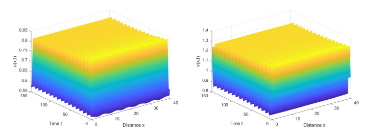
Figure 1.
Turing instability of periodic solution fails.
Extension professionals are expected to help disseminate agricultural technologies, information, knowledge and skills to farmers. In order to develop valuable and long-lasting extension services, it is essential to understand the methods of extension that farmers find most beneficial. This understanding helps adopt improved practices, overcome barriers, provide targeted interventions and continuously improve agricultural extension programs. Thus, assessing factors affecting farmers' choice of agricultural extension methods is essential for developing extension methods that comply with farmers' needs and socio-economic conditions. Therefore, we analyzed the factors affecting farmers' preferences in extension methods, using cross-sectional data collected from 300 households in two sample districts and 16 Kebelles in Ethiopia between September 2019 and March 2020. Four extension methods, including training, demonstration, office visits and phone calls were considered as outcome variables. We fitted a multivariate probit model to estimate the factors that influence farmers' choice of extension methods. The results of the study showed that the number of dependents in the household head, formal education and membership of Idir (an informal insurance program a community or group runs to meet emergencies) were negatively associated with farmers' choices to participate in different extension methods compared to no extension. On the other hand, the sex of the household head, farm experience, participation in non-farm activities, monetary loan access, owning a mobile phone, radio access and membership of cooperatives were found to have a statistically significant positive impact on farmers' choices of extension methods. Based on these findings, the government and the concerned stakeholders should take farmers' socio-economic and institutional traits into account when selecting and commissioning agricultural extension methods. This could help to develop contextually relevant extension strategies that are more likely to be chosen and appreciated by farmers. Furthermore, such strategies can aid policymakers in designing extension programs that cater to farmers' needs and concerns. In conclusion, farmers' socio-economic and institutional affiliation should be taken into consideration when selecting agricultural extension methods.
Citation: Yemane Asmelash Gebremariam, Joost Dessein, Beneberu Assefa Wondimagegnhu, Mark Breusers, Lutgart Lenaerts, Enyew Adgo, Steven Van Passel, Amare Sewnet Minale, Amaury Frankl. Listen to the radio and go on field trips: A study on farmers' attributes to opt for extension methods in Northwest Ethiopia[J]. AIMS Agriculture and Food, 2024, 9(1): 3-29. doi: 10.3934/agrfood.2024002
| [1] | Zizhuo Wu, Qingshan She, Zhelong Hou, Zhenyu Li, Kun Tian, Yuliang Ma . Multi-source online transfer algorithm based on source domain selection for EEG classification. Mathematical Biosciences and Engineering, 2023, 20(3): 4560-4573. doi: 10.3934/mbe.2023211 |
| [2] | Xia Chen, Yexiong Lin, Qiang Qu, Bin Ning, Haowen Chen, Xiong Li . An epistasis and heterogeneity analysis method based on maximum correlation and maximum consistence criteria. Mathematical Biosciences and Engineering, 2021, 18(6): 7711-7726. doi: 10.3934/mbe.2021382 |
| [3] | Bo Wang, Yabin Li, Xue Sui, Ming Li, Yanqing Guo . Joint statistics matching for camera model identification of recompressed images. Mathematical Biosciences and Engineering, 2019, 16(5): 5041-5061. doi: 10.3934/mbe.2019254 |
| [4] | Shi Liu, Kaiyang Li, Yaoying Wang, Tianyou Zhu, Jiwei Li, Zhenyu Chen . Knowledge graph embedding by fusing multimodal content via cross-modal learning. Mathematical Biosciences and Engineering, 2023, 20(8): 14180-14200. doi: 10.3934/mbe.2023634 |
| [5] | Pingping Sun, Yongbing Chen, Bo Liu, Yanxin Gao, Ye Han, Fei He, Jinchao Ji . DeepMRMP: A new predictor for multiple types of RNA modification sites using deep learning. Mathematical Biosciences and Engineering, 2019, 16(6): 6231-6241. doi: 10.3934/mbe.2019310 |
| [6] | Ting-Huai Ma, Xin Yu, Huan Rong . A comprehensive transfer news headline generation method based on semantic prototype transduction. Mathematical Biosciences and Engineering, 2023, 20(1): 1195-1228. doi: 10.3934/mbe.2023055 |
| [7] | Shizhen Huang, ShaoDong Zheng, Ruiqi Chen . Multi-source transfer learning with Graph Neural Network for excellent modelling the bioactivities of ligands targeting orphan G protein-coupled receptors. Mathematical Biosciences and Engineering, 2023, 20(2): 2588-2608. doi: 10.3934/mbe.2023121 |
| [8] | Jun Yan, Tengsheng Jiang, Junkai Liu, Yaoyao Lu, Shixuan Guan, Haiou Li, Hongjie Wu, Yijie Ding . DNA-binding protein prediction based on deep transfer learning. Mathematical Biosciences and Engineering, 2022, 19(8): 7719-7736. doi: 10.3934/mbe.2022362 |
| [9] | Sarth Kanani, Shivam Patel, Rajeev Kumar Gupta, Arti Jain, Jerry Chun-Wei Lin . An AI-Enabled ensemble method for rainfall forecasting using Long-Short term memory. Mathematical Biosciences and Engineering, 2023, 20(5): 8975-9002. doi: 10.3934/mbe.2023394 |
| [10] | M Kumaresan, M Senthil Kumar, Nehal Muthukumar . Analysis of mobility based COVID-19 epidemic model using Federated Multitask Learning. Mathematical Biosciences and Engineering, 2022, 19(10): 9983-10005. doi: 10.3934/mbe.2022466 |
Extension professionals are expected to help disseminate agricultural technologies, information, knowledge and skills to farmers. In order to develop valuable and long-lasting extension services, it is essential to understand the methods of extension that farmers find most beneficial. This understanding helps adopt improved practices, overcome barriers, provide targeted interventions and continuously improve agricultural extension programs. Thus, assessing factors affecting farmers' choice of agricultural extension methods is essential for developing extension methods that comply with farmers' needs and socio-economic conditions. Therefore, we analyzed the factors affecting farmers' preferences in extension methods, using cross-sectional data collected from 300 households in two sample districts and 16 Kebelles in Ethiopia between September 2019 and March 2020. Four extension methods, including training, demonstration, office visits and phone calls were considered as outcome variables. We fitted a multivariate probit model to estimate the factors that influence farmers' choice of extension methods. The results of the study showed that the number of dependents in the household head, formal education and membership of Idir (an informal insurance program a community or group runs to meet emergencies) were negatively associated with farmers' choices to participate in different extension methods compared to no extension. On the other hand, the sex of the household head, farm experience, participation in non-farm activities, monetary loan access, owning a mobile phone, radio access and membership of cooperatives were found to have a statistically significant positive impact on farmers' choices of extension methods. Based on these findings, the government and the concerned stakeholders should take farmers' socio-economic and institutional traits into account when selecting and commissioning agricultural extension methods. This could help to develop contextually relevant extension strategies that are more likely to be chosen and appreciated by farmers. Furthermore, such strategies can aid policymakers in designing extension programs that cater to farmers' needs and concerns. In conclusion, farmers' socio-economic and institutional affiliation should be taken into consideration when selecting agricultural extension methods.
In nonlinear chemical reaction systems, the three-molecule autocatalytic model shows abundant dynamical behaviors, many abundant research results have been obtained [1,2,3,4,5,6,7]. In 1979, Schnakenberg proposed a typical three-molecule autocatalytic reaction-diffusion model [8]. In [9], the authors studied the one-dimensional static Turing bifurcation of Schnakenberg model. In [10,11,12], the authors introduced the relevant research background of reaction-diffusion Schnakenberg system. However, most references [13,14,15,16] focus on whether the constant equilibrium solution has Turing instability, but pay little attention to whether the periodic solutions of system may also suffer from Turing instability. Therefore, by applying the theoretical methods in [17,18], we study the Turing instability of Hopf bifurcating periodic solutions for the Schnakenberg model.
On the basis of the Schnakenberg model [8], We introduce self-diffusion and cross-diffusion coefficients, and establish reaction-diffusion Schnakenberg model with cross-diffusion and self-diffusion:
| {ut−d11Δu−d12Δv=a−u+u2v,x∈Ω,t>0,vt−d21Δv−d22Δv=b−u2v,x∈Ω,t>0,u(x,0)=u∗(x),v(x,0)=v∗(x),x∈Ω,∂u∂ν=∂v∂ν=0,x∈∂Ω,t>0, | (1.1) |
where Ω is a open bounded domain in n-dimensional Euclidean space, and its boundary ∂Ω is smooth. Δ is Laplace operator. The parameters a,b,d11,d12,d21,d22 are all positive constants. u=u(x,t) and v=v(x,t) indicate the concentrations of chemicals at position x∈Ω and time t>0, respectively, and the initial concentrations u∗(x),v∗(x) are nonnegative functions. d11,d22 denote self-diffusion coefficients of u and v, respectively. d12,d21 represent cross-diffusion coefficients of u and v, respectively. Simultaneously, we suppose that d11d22−d12d21>0 holds.
We consider the corresponding zero-dimensional dynamic system of system (1.1)
| {dudt=a−u+u2v, t>0,dvdt=b−u2v, t>0,u(0)=u∗>0,v(0)=v∗>0. | (2.1) |
The equilibrium (u0,v0) of system (2.1) satisfies
| {a−u+u2v=0,b−u2v=0. |
with u0=a+b,v0=b(a+b)2. By straightforward computation, we know (u0,v0) is the only equilibrium of system (2.1). For convenience, setting μ:=a+b, then (u0,v0)=(μ,bμ2). In the following, for the three-molecule autocatalytic Schnakenberg model, we discuss the stability of its Hopf bifurcating periodic solutions by taking μ as parameter.
Theorem 2.1. Let μH0=3√b+√b2+127+3√b−√b2+127, for the ODEs (2.1), the following statements are true:
(1) At (μ,bμ2)T, system (2.1) is unstable for μ∈(0,μH0), while locally asymptotically stable for μ∈(μH0,+∞).
(2) At λ=μH0, system has a family of periodic solutions (uT(t),vT(t))T bifurcating from (μ,bμ2)T. Supercritical Hopf bifurcation of system (2.1) occurs at (μ,bμ2)T, and the bifurcating periodic solutions are stable.
Proof. The Jacobian matrix of system (2.1) at (μ,vμ)T is J(μ)=(−1+2bμμ2−2bμ−μ2). The characteristic equation of J(μ) is
| λ2−T(μ)λ+D(μ)=0, | (2.2) |
with
| T(μ)=−μ2−1+2bμ,D(μ)=μ2. |
The eigenvalue λ(μ) of J(μ) is given by
| λ(μ)=T(μ)±√T2(μ)−4D(μ)2. |
When μ≥2b, all the eigenvalues of J(μ) have strict negative real parts, according to the stability theory, the equilibrium (μ,bμ2)T is locally asymptotically stable. When 0<μ<2b, T′(μ)=−2μ−2bμ2<0, then T(μ) is monotonically decreasing for 0<μ<2b. Since limμ→0T(μ)=+∞,T(2b)=−4b−12b<0, then T(μ) has only zero point μH0∈(0,2b), namely, T(μH0)=0. For any μ∈(μH0,2b), we have T(μ)<0, then system (2.1) is locally asymptotically stable at (μ,bμ2)T, while for any μ∈(0,μH0), system (2.1) is unstable at (μ,bμ2)T. When μ=μH0, J(μ) has a pair of pure imaginary roots λ=±iω0 with ω0=μ. Let λ(μ)=α(μ)±iω(μ) be the roots of Eq (2.2) near μ=μH0, then we have
| α(μ)=−μ22−12+bμ,dα(μ)dμ|μ=μH0<0. |
According to Poincaré-Andronov-Hopf bifurcation theorem, system (2.1) experiences a Hopf bifurcation at μ=μH0.
Next, we study the properties of Hopf bifurcating periodic solutions of system (2.1). Here, we still use the notations and computation in [20] to deduce the expression of cubic term coefficient c1(μH0) in the norm form. By [21], we can rewrite the Poincaré normal form of the abstract form of system (2.1) in the small neighborhood of p0 as follows:
| dUdt=J(μH0)U+F(μ,U)|μ=μH0. | (2.3) |
Let the eigenvector of J(μH0) corresponding to the eigenvalue iω0 be q=(a0,b0)T satisfying
| J(μH0)q=iω0q,q=(a0,b0)T=(−μH0,μH0−i)T. |
Define inner product in XC:
| ⟨U1,U2⟩=∫lπ0(ˉu1u2+ˉv1v2)dx, |
where Ui=(ui,vi)T∈XC,i=1,2. Note that ⟨λU1,U2⟩=ˉλ⟨U1,U2⟩, denote the adjoint operator of J(μH0) by J∗(μH0), then the eigenvector of J∗(μH0) corresponding to the eigenvalue −iω0 be q∗=(a∗0,b∗0)T∈XC satisfying
| J∗(μH0)q∗=−iω0q∗,<q∗,q>=1,<q∗,ˉq>=0. |
Therefore, q∗=(a∗0,b∗0)T=(−1−iμH02μH0lπ,−i2lπ)T. Performing the spatial decomposition X=Xc⊕Xs, where Xc={zq+ˉzˉq|z∈C},Xs={u∈X|<q∗,u>=0}, then for any U=(u,v)T∈X, there exist z∈C and ω=(ω1,ω2)∈Xs such that (u,v)T=zq+ˉzˉq+(ω1,ω2)T. Thus, system (2.3) can be transformed into the following system with (z,ω) as the coordinate:
| {dzdt=iωz+<q∗,F(p,U)|p=p0>,dωdt=L(p0)ω+H(z,ˉz,ω), | (2.4) |
with
| {H(z,ˉz,ω)=F(p,U)|p=p0−<q∗,F(p,U)|p=p0>q−<ˉq∗,F(p,U)|p=p0>ˉq,F(p,U)|p=p0=F0(zq+ˉzˉq+ω). | (2.5) |
Writing F0 as
| F0(U)=12Q(U,U)+16C(U,U,U)+O(|U|4), | (2.6) |
here, Q,C is a symmetric multilinear form. For convenience, denoting QXY=Q(X,Y),CXYZ=C(X,Y,Z), we calculate Qqq, Qqˉq and Cqqˉq, where
| Qqq=(c0d0),Qqˉq=(e0f0),Cqqˉq=(g0h0), |
here, denoting f(u,v)=a−u+u2v,g(u,v)=b−u2v, with
| c0=fuua20+2fuva0b0+fvvb20=μH0−3μH03+4μH02i,d0=guua20+2guva0b0+gvvb20=−c0=−μH0+3μH03−4μH02i,e0=fuu|a0|2+fuv(a0¯b0+¯a0b0)+fvv|b0|2=μH0−3μH03,f0=guu |a0|2+guv (a0¯b0+¯a0b0)+gvv|b0|2=−e0=3μH03−μH0,g0=fuuu |a0|2a0+fuuv (2|a0|2b0+a20¯b0)+fuvv(2|b0|2a0+b20¯a0)a=6μH03−2μH02i,h0=guuu |a0|2a0+guuv (2|a0|2b0+a20¯b0)+guvv(2|b0|2a0+b20¯a0)=−g0=−6μH03+2μH02i, |
here, all the partial derivatives of f(u,v) and g(u,v) are evaluated at the bifurcation point (μH0,bμH02)T,
Let
| H(z,ˉz,ω)=H202z2+H11zˉz+H022ˉz2+o(|z|3)+o(|z||ω|), | (2.7) |
from (2.5) and (2.6), we can obtain
| {H20=Qqq−<q∗,Qqq>q−<ˉq∗,Qqq>ˉqH11=Qqˉq−<q∗,Qqˉq>q−<ˉq∗,Qqˉq>ˉq |
Because system (2.4) has normal manifold, which can be written as follows
| ω=ω202z2+ω11zˉz+ω022ˉz2+o(|z|3). | (2.8) |
By (2.7), (2.8) and J(μH0)ω+H(z,ˉz,ω)=dωdt=∂ω∂zdzdt+∂ω∂ˉzdˉzdt, we have
| ω20=(2iω0I−J(μH0))−1H20,ω11=−J−1(μH0)H11. |
By calculation, we have
| <q∗,Qqq>=−c02μH0=−μH0+3μH03−4μH02i2μH0,<q∗,Qqˉq>=−e02μH0=−μH0+3μH032μH0,<ˉq∗,Cqqˉq>=−g02μH0=−6μH03+2μH02i2μH0,<ˉq∗,Qqq>=−c02μH0=−μH0+3μH03−4μH02i2μH0,<ˉq∗,Qqˉq>=−e02μH0=−μH0+3μH032μH0, |
we can also get H20=0,H11=0, this implies ω20=ω11=0, then
| <q∗,Qω11q>=<q∗,Qω20ˉq>=0. |
Thus, we have
| c1(μ)=i2ω0<q∗,Qqq>⋅<q∗,Qqˉq>+12<ˉq∗,Cqqˉq>. |
The real part and imaginary part of c1(μH0) are as follows
| Rec1(μH0)=Re{i2ω0<q∗,Qqq>⋅<q∗,Qqˉq>+12<ˉq∗,Cqqˉq>}=−12,Imc1(μH0)=Im{i2ω0<q∗,Qqq>⋅<q∗,Qqˉq>+12<ˉq∗,Cqqˉq>}=18μH0−μH04+9μH038. | (2.9) |
By Rec1(μH0)<0, we know that the Hopf bifurcating periodic solutions of system (2.1) are stable at μ=μH0. Additionally, because transversality condition dα(μ)dμ|μ=μH0<0, so the direction of Hopf bifurcation is subcritical.
We introduce the following perturbed system model on the basis of ODEs (2.1)
| (1+εd11εd12εd211+εd22)(dudt,dvdt)T=(a−u+u2vb−u2v), | (2.10) |
here, ε is sufficiently small such that (1+εd11εd12εd211+εd22) is reversible. System (2.10) is equivalent to the following system
| (dudt,dvdt)T=1N(ε)(1+d22ε−d12ε−d21ε1+d11ε)(a−u+u2vb−u2v), | (2.11) |
where
| N(ε):=|(1+d22ε−d12ε−d21ε1+d11ε)|=(d11d22−d12d21)ε2+(d11+d22)ε+1>0. |
Then at (μ,vμ), the Jacobian matrix of system (2.11) is
| J(μ,ε):=1N(ε)(a11(μ,ε)a12(μ,ε)a21(μ,ε)a22(μ,ε)), | (2.12) |
with
| a11(μ,ε):=(1+d22ε)(−1+2bμ)+d12ε2bμ,a12(μ,ε):=(1+d22ε)μ2+d12εμ2,a21(μ,ε):=−(1+d11ε)2bμ−d21ε(−1+2bμ),a22(μ,ε):=−μ2(1+d11ε)−d21εμ2. | (2.13) |
The characteristic equation corresponding to the jacobian matrix J(μ,ε) is
| λ2−H(μ,ε)λ+D(μ,ε)=0, | (2.14) |
where
| H(μ,ε)=1N(ε)[(2bμ−1−μ2)+ε(d22(2bμ−1)−μ2d11+d12⋅2bμ−d21⋅μ2)],D(μ,ε)=μ2N(ε). | (2.15) |
Notice that H(μH0,0)=T(μH0)=0 and ∂μH(μ,ε)=T′(μH0)≠0. According to the implicit function existence theorem, there exist a sufficiently small ε0>0 and a continuously differentiable function μHε=μH(ε) such that when ε∈(−ε0,ε0), H(μHε,ε)=0 and μH(0)=μH0 hold. Let λ(με)=β(με)±iω(με) be the characteristic root of Eq 2.14, then when μ→με, we have
| β(με)=12H(μ,ε),ω(με)=12√4D(μ,ε)−H2(μ,ε). | (2.16) |
By [18], we have the following lemma.
Lemma 2.1. Assume μ is sufficiently close to μHε, T is the minimum positive period of the stable periodic solution (uT(t),vT(t)) of system (2.1) bifurcating from (μ,vμ), then there exists ε1>0 such that for any ε∈(−ε1,ε1), system (2.10) has a periodic solution (uT(t,ε),vT(t,ε)) depending on ε. Its minimum positive period is T(ε), simultaneously, it satisfies
1) When ε→0, (uT(t,ε),vT(t,ε))→(uT(t),vT(t)) and T(ε)→T.
2) T(ε)=2πω(μHε)(1+(β′(μHε)Im(c1(μHε))ω(μHε)Re(c1(μHε))−ω′(μHε)ω(μHε))(μ−μHε)+O((μ−μHε)2) with
| c1(μHε)=i2ω(μHε)(g20(ε)g11(ε)−2|g11(ε)|2−13|g02(ε)|2)+g21(ε)2. |
Theorem 2.2. Suppose that μ is sufficiently close to μHε, (uT(t),vT(t)) is the stable periodic solution of system (2.1), then when ε→0, we have
| T′(0)=πμH0(L1(μH0)d11−L2(μH0)d22−L3(μH0)d12−L4(μH0)d21), |
with
| L1(μH0)=54−μH202+9μH404,L2(μH0)=(14μH20+9μH204−1)(2bμH0−1)−1,L3(μH0)=(14μH0+9μH304−μH0)2bμH20,L4(μH0)=(μH0−14μH0−9μH304)μH0. |
Proof. According to Lemma 2.1, we have
| T′(ε)=−2πω2(μHε)dω(μHε)dε−2πω(μHε)(β′(μHε)Im(c1(μHε))ω(μHε)Re(c1(μHε))−ω′(μHε)ω(μHε))dμHεdε+O(μ−μHε). |
If μ→μHε, then O(μ−μHε)→0, so the sign of T′(ε) is mainly determined by the sign of the first two at ε=0. Next, we calculate the expressions of dμHεdε|ε=0 and dω(μHε)dε|ε=0.
At μ=μHε, by (2.15), we can derive
| (2bμHε−1−μHε2)+ε(d22(−1+2bμHε)−μHε2d11+d122bμHε−d21μHε2)=0. | (2.17) |
Differentiating (2.17) with ε, we have
| dμHεdε|ε=0=b(μH0)2bμH02+2μH0, | (2.18) |
with
| b(μH0)=d22(−1+2bμH0)−μH02d11+d122bμH0−d21μH02. | (2.19) |
According to (2.16),
| ω(μ)=12√4D(μ,ε)−H2(μ,ε). |
Differentiating it with μ, we know
| ω′(μ)=∂μD(μ,ε)−12H(μ,ε)∂μH(μ,ε)√4D(μ,ε)−H2(μ,ε). |
When μ→μHε, H(μHε,ε)=0 and ∂λD(μHε,ε)=1N(ε)D′(μHε). Hence,
| ω′(μH0)=∂λD(μHε,ε)2√D(μHε,ε)|ε=0=D′(μHε)2√N(ε)D(μHε)|ε=0=D′(μ)2√D(μ). | (2.20) |
From ω(μHε)=√D(μHε,ε) and D(μHε,ε)=D(μHε)N(ε), differentiating them with ε, we can obtain
| dω(μHε)dε=12√D(μHε,ε)ddε(D(μHε,ε)). | (2.21) |
| ddε(D(μHε,ε))=−N′(ε)N2(ε)D(μHε)+ddε(D(μHε))1N(ε). | (2.22) |
When ε=0, we get
| −N′(0)N2(0)D(μH0)=−(d11+d22)D(μH0),ddε(D(μHε))1N(ε)|ε=0=D′(μ0)dμHεdε(0). | (2.23) |
Thus, according to (2.22) and (2.23), we have
| ddε(D(μHε,ε))|ε=0=−(d11+d22)D(μH0)+b(μH0)2bμH02+2μH0D′(μH0), | (2.24) |
where b(μH0) is defined in (2.19). From (2.21) and (2.24), we can obtain
| ddε(ω(μHε))|ε=0=−12√D(μH0)(d11+d22−b(μH0)2bμH02+2μH0D′(μH0)D(μH0)). | (2.25) |
By (2.18), (2.20) and (2.25), we can deduce
| T′(0)=πD(μH0)(√D(μH0)d11+√D(μH0)d22+b(μH0)Im(c1(μH0))Re(c1(μH0))). | (2.26) |
At last, substituting (2.19) into (2.26), we can obtain
| T′(0)=πμH0(L1(μH0)d11−L2(μH0)d22−L3(μH0)d12−L4(μH0)d21), |
with
| L1(μH0)=54−μH202+9μH404,L2(μH0)=(14μH20+9μH204−1)(2bμH0−1)−1,L3(μH0)=(14μH0+9μH304−μH0)2bμH20,L4(μH0)=(μH0−14μH0−9μH304)μH0. |
In this section, applying the theory elaborated in [17], we study stable spatially homogeneous Hopf bifurcating periodic solutions of system (2.1) will become Turing unstable in reaction-diffusion system (1.1) with cross-diffusion. According to the previous discussion, we give the following theorem.
Theorem 3.1. Suppose that μ is sufficiently close to μ0, (uT(t),vT(t)) is stable spatially homogeneous Hopf bifurcating periodic solution of system (2.1) bifurcating from (μ,vμ). If T′(0)<0 and Ω is large enough, then (uT(t),vT(t)) will become Turing unstable in system (1.1) with cross-diffusion.
Proof. Assume that the stable periodic solution of system (2.1) is (uT(t),vT(t)) with minimum positive period T, then the linearized system of (1.1) evaluated at (uT(t),vT(t)) is
| (∂ϕ∂t,∂φ∂t)T=diag(DΔϕ,D Δ φ)+JT(t)(ϕ,φ)T, | (3.1) |
where D:=(d11d12d21d22), Δ is Laplace operator, the Jacobian matrix of system (2.1) at (uT(t),vT(t)) is JT(t):=(−1+2uT(t)vT(t)uT2(t)−2uT(t)vT(t)−uT2(t)). Setting βn and ηn(x) be the eigenvalue and eigenfunction of −Δ in Ω with Neumann boundary condition. Let (ϕ,φ)T=(h(t),g(t))T∑∞n=0knηn(x), then
| (dhdt,dgdt)T=−τD(h(t)g(t))+JT(t)(h(t)g(t)), | (3.2) |
in which, τ:=βn≥0,n∈N0:={0,1,2⋯}. Assume d11=d12=d21=d22=0, then system (3.2) can be rewritten as
| (dhdt,dgdt)T=JT(t)(h(t),g(t))T. | (3.3) |
Let Φ(t) be the fundamental solution matrix of system (3.3) satisfying Φ(0)=I2. Denote λi,i=1,2 as the eigenvalue of Φ(T), the corresponding characteristic function is (Ni,Mi)T, i.e.,
| Φ(T)(Ni,Mi)T=λi(Ni,Mi)T, |
then λi is the Floquet multiplier corresponding to the periodic solution (uT(t),vT(t)) of system (3.2). Define
| (ϕi(t),ψi(t))T:=Φ(t)(Ni,Mi)T, |
apparently,
| (ϕi(0),ψi(0))T=(Ni,Mi)T,Φ(T)(ϕi(0),ψi(0))T=λi(ϕi(0),ψi(0))T. |
In system (2.1), differentiating with t, we have
| (du′dt,dv′dt)T=(−1+2uvu2−2uv−u2)(u′v′). |
Then 1 is the eigenvalue of Φ(T), the corresponding eigenvector is (u′T(0),v′T(0))T. We might as well assume λ1=1, (ϕ1(t),ψ1(t))T=(u′T(t),v′T(t))T. Since (uT(t),vT(t)) is stable, then |λ2|<1. Let Φ(t,τ) be the fundamental solution matrix of system (3.2), and Φ(0,τ)=I, namely,
| ∂Φ(t,τ)∂t=−τDΦ(t,τ)+JT(t)Φ(t,τ). |
For sufficiently small τ, Φ(t,τ) is continuously differentiable with respect to t and τ, and Φ(t,0)=Φ(t). Define mapping L:[0,+∞)×C×C2→C2, where C:=R⊕iR, we have
| L(τ,δi,(nimi)):=Φ(T,τ)(nimi)−δi(nimi), |
clearly, L(0,λi,(Ni,Mi)T)=(0,0)T and
| Lδi(0,λi,(Ni,Mi)T)=−(Ni,Mi)T,L(ni,mi)T(0,λi,(Ni,Mi)T)=Φ(T)−λiI, |
here, Lδi is the Fréchet derivative of L with respect to δi, and L(ni,mi)T is the Fréchet derivative of L with respect to (ni,mi)T. Setting λi is the single eigenvalue of Φ(T), then we have
| Ker(λiI−Φ(T))=span{(Ni,Mi)T},(Ni,Mi)T∉Rank(λiI−Φ(T)). |
where Ker represents the kernel of λiI−Φ(T), and Rank represents the range of λiI−Φ(T), then L(δi,(ni,mi)T)(0,λi,(Ni,Mi)T),i=1,2 is an isomorphic mapping. By the implicit function theorem, there exist τ1>0, τ∈(−τ1,τ1) and continuously differentiable functions δi(τ),ni(τ),mi(τ) such that
| Φ(T,τ)(ni(τ),mi(τ))T=δi(τ)(ni(τ),mi(τ))T, | (3.4) |
where δi(τ),i=1,2 are the Floquet multipliers corresponding to (uT(t),vT(t)). Define
| (ϕi(t,τ),ψi(t,τ))T:=Φ(t,τ)(ni(τ),mi(τ))T, | (3.5) |
by Φ(0,τ)=I and (3.5), we can obtain
| (ϕi(0,τ),ψi(0,τ))T=(ni(τ),mi(τ))T. | (3.6) |
From (3.4) and (3.6), we have
| Φ(T,τ)(ϕi(0,τ),ψi(0,τ))T=δi(τ)(ϕi(0,τ),ψi(0,τ))T. |
Specifically, by (3.5), we have
| (ϕi(t,0),ψi(t,0))T=Φ(t,0)(ni(0),mi(0))T=Φ(t)(Ni,Mi)T, =Φ(t)(ϕi(0),ψi(0))T=(ϕi(t),ψi(t))T. | (3.7) |
By the definition of (ϕ1(t,τ),ψ1(t,τ))T in (3.5), we can obtain
| (∂ϕ1(t,τ)∂t,∂ψ1(t,τ)∂t)T=−τD(ϕ1(t,τ),ψ1(t,τ))T+JT(t)(ϕ1(t,τ),ψ1(t,τ))T. | (3.8) |
Differentiating (3.8) with respect to τ and setting τ=0, we have
| (∂ϕ1τ(t,0)∂t,∂ψ1τ(t,0)∂t)T=−D(ϕ1(t),ψ1(t))T+JT(t)(ϕ1τ(t,0),ψ1τ(t,0))T, | (3.9) |
here, ϕ1τ:=∂τϕ1,ψ1τ:=∂τψ1. On the other hand, from (3.4) and (3.5), we can derive
| (ϕ1(T,τ),ψ1(T,τ))T=δ1(τ)(ϕ1(0,τ),ψ1(0,τ))T. | (3.10) |
Differentiating (3.10) with τ, we get
| (ϕ1τ(T,τ),ψ1τ(T,τ))T=δ′1(τ)(ϕ1(0,τ),ψ1(0,τ))T+δ1(τ)(ϕ1τ(0,τ),ψ1τ(0,τ))T. | (3.11) |
In (3.11), setting τ=0, from (3.6)and δ1(0)=λ1=1, we have
| (ϕ1τ(T,0),ψ1τ(T,0))T=δ′1(0)(ϕ1(0),ψ1(0))T+(ϕ1τ(0,0),ψ1τ(0,0))T. | (3.12) |
According to Lemma 2.1, (uT(t,ε),vT(t,ε)) is the periodic solution of system (2.10), that is,
| (I+εD)(∂uT(t,ε)∂t,∂uT(t,ε)∂t)T=(a−uT(t,ε)+uT2(t,ε)vT(t,ε)b−uT2(t,ε)vT(t,ε)). | (3.13) |
Differentiating (3.13) with respect to ε and setting ε=0, we have
| (d(∂tuT(t,0))dε,d(∂tvT(t,0))dε)T=−D(ϕ1(t),ψ1(t))T+JT(t)(duT(t,0)dε,dvT(t,0)dε)T, | (3.14) |
where ∂tuT(t,0)=ϕ1(t),∂tvT(t,0)=ψ1(t). Since (uT(t,ε),vT(t,ε)) is the periodic solution with period T(ε), thus,
| (uT(t,ε),vT(t,ε))T=(uT(t+T(ε),ε),vT(t+T(ε),ε))T. | (3.15) |
In (3.15), differentiating with respect to ε and setting ε=0,t=0, then
| (duT(T,0)dε,dvT(T,0)dε)T=−T′(0)(ϕ1(0),ψ1(0))T+(duT(0,0)dε,dvT(0,0)dε)T, | (3.16) |
here, uT(t,0)=uT(t),vT(t,0)=vT(t),T(0)=T. Define
| Γ(t):=(ϕ1τ(t,0),ψ1τ(t,0))T−(duT(t,0)dε,dvT(t,0)dε)T. |
From (3.9), (3.12), (3.14) and (3.16), we have
| ddtΓ(t)=JT(t)Γ(t), | (3.17) |
| Γ(T)−Γ(0)=(δ′1(0)+T′(0))(ϕ1(0),ψ1(0))T. | (3.18) |
Let Γ(t)=Φ(t)(Y1,Y2)T be the general solution of (3.17), where any vector (Y1,Y2)T∈R2. Since (ϕ1(0),ψ1(0))T and (ϕ2(0),ψ2(0))T are linearly independent, then there exit constants γ1 and γ2 so that
| (Y1,Y2)T=γ1(ϕ1(0),ψ1(0))T+γ2(ϕ2(0),ψ2(0))T. | (3.19) |
Substituting (3.19) into (3.18), we can obtain δ′1(0)+T′(0)=0. Assume that T′(0)<0, which is equivalent to δ′1(0)>0, if Ω is large enough so that the minimum positive eigenvalue of −Δ is small enough, then there exists at least one eigenvalue βn of −Δ such that δ1(τ)=δ1(βn)>1. Thus, (uT(t),vT(t)) becomes Turing unstable in reaction-diffusion system (1.1) with cross-diffusion.
In this section, we shall select several groups of data for numerical simulations to support theoretical analysis. In system (1.1), Fix parameters a=0.1823,b=0.5, initial values u0=0.6+0.01cosx,v0=1+0.01sinx, then the equilibrium is (0.6823,1.074), μH0=0.6823278, Rec1(μH0)=−0.5<0, Imc1(μH0)=−0.0270945<0. According to Theorem 2.1, system (2.1) produces a spatially homogeneous Hopf bifurcating periodic solution (uT(t),vT(t))T at the equilibrium, which is stable and subcritical. By calculation, we can obtain
| L1(μH0)=1.50492,L2(μH0)=−0.72787,L3(μH0)=0.85664,L4(μH0)=−0.27213. |
For different diffusion coefficients, Turing instability of system (1.1) at the periodic solution (uT(t),vT(t))T is different. Hence, we give diffusion coefficients in four cases and carry out corresponding numerical simulations.
(1) If we select d11=1,d22=1,d12=d21=0, at this moment, Turing instability of (uT(t),vT(t))T does not exist in system (1.1) (Figure 1). That is, the same diffusion rates will not cause Turing instability of periodic solution ([19]).
(2) If we select d11=0.05,d22=2,d12=d21=0, then
| L1(μH0)d11+L2(μH0)d22−L3(μH0)d12−L4(μH0)d21<0. |
According to Theorem 3.1, system (1.1) is Turing unstable at periodic solution (uT(t),vT(t))T. Through simulation simulation, it can be observed that the stable periodic solution produces Turing bifurcation (Figure 2), which is consistent with the theoretical analysis.

(3) If we choose d11=d22=1,d21=0.2,d12=1.05, from Theorem 3.1, we have
| L1(μH0)d11+L2(μH0)d22−L3(μH0)d12−L4(μH0)d21<0, |
then system (1.1) is Turing unstable at periodic solution (uT(t),vT(t))T. Through simulation simulation, it can be verified that the stable periodic solution generates Turing bifurcation (Figure 3). Therefore, cross-diffusion causes the stable periodic solution of system (1.1) to become Turing unstable. self-diffusion induces Turing instability of periodic solution.

(4) If we choose d11=0.5,d12=1.5,d21=0.6,d22=4, then
| L1(μH0)d11+L2(μH0)d22−L3(μH0)d12−L4(μH0)d21<0. |
By Theorem 3.1, we can derive that diffusion causes the stable periodic solution of system (1.1) to become Turing unstable (Figure 4). This conforms to the theoretical analysis.

In this paper, a three-molecule autocatalytic Schnakenberg model with cross-diffusion is considered. From both theoretical and numerical perspectives, we investigated how cross-diffusion causes the Turing instability of spatially homogeneous Hopf bifurcating periodic solutions.
The theoretical results indicate that in the Schnakenberg model, when the parameters satisfy certain conditions and Ω is sufficiently large, once the instability of periodic solutions induced by diffusion occurs, new and rich spatiotemporal patterns may emerge. For the reaction-diffusion Schnakenberg model, we can derive the precise conditions of diffusion rates, under which the periodic solutions may experience the instability caused by diffusion.
By numerical simulations, the Turing instability of periodic solution (uT(t),vT(t))T can be observed. Figure 1 shows that without cross-diffusion coefficients, the identical self-diffusion coefficients will not cause the stable periodic solution to produce Turing bifurcation. Figures 2 and 4 illustrate that with appropriate diffusion coefficients, the stable periodic solution of system (1.1) generates Turing instability. Figure 3 indicates that if we select appropriate cross-diffusion coefficients, even for the models with identical self-diffusion rates, cross-diffusion can also cause stable periodic solution to produce Turing bifurcation. Thus, the Turing instability of stable periodic solution (uT(t),vT(t))T is actually induced by cross-diffusion.
The authors declare there is no conflicts of interest.
| [1] | Albore A (2018) Review on role and challenges of agricultural extension service on farm productivity in Ethiopia. Int J Agric Educ Ext 4: 93–100. |
| [2] | Elias A, Nohmi M, Yasunobu K, et al. (2016) Farmers' satisfaction with agricultural extension service and its influencing factors: a case study in North West Ethiopia. J Agric Sci Technol 18: 39–53. |
| [3] |
Mutengwa CS, Mnkeni P, Kondwakwenda A (2023) Climate-smart agriculture and food security in Southern Africa: A review of the vulnerability of smallholder agriculture and food security to climate change. Sustainability 15: 2882. https://doi.org/10.3390/su15042882 doi: 10.3390/su15042882

|
| [4] | Swanson BE, Rajalahti R (2010) Strengthening agricultural extension and advisory systems: Procedures for assessing, transforming, and evaluating extension systems. Agriculture and Rural Development Discussion Paper, No. 45. World Bank, Washington, DC. |
| [5] |
Takahashi K, Muraoka R, Otsuka K (2020) Technology adoption, impact, and extension in developing countries' agriculture: A review of the recent literature. Agric Econ 51: 31–45. https://doi.org/10.1111/agec.12539 doi: 10.1111/agec.12539
|
| [6] |
Mapiye O, Makombe G, Molotsi A, et al. (2021) Towards a revolutionized agricultural extension system for the sustainability of smallholder livestock production in developing countries: The potential role of icts. Sustainability 13: 5868. https://doi.org/10.3390/su13115868 doi: 10.3390/su13115868
|
| [7] |
Norton GW, Alwang J (2020) Changes in agricultural extension and implications for farmer adoption of new practices. Appl Econ Perspect Policy 42: 8–20. https://doi.org/10.1002/aepp.13008 doi: 10.1002/aepp.13008
|
| [8] |
Faure G, Desjeux Y, Gasselin P (2012) New challenges in agricultural advisory services from a research perspective: A literature review, synthesis and research agenda. J Agric Educ Ext 18: 461–492. https://doi.org/10.1080/1389224X.2012.707063 doi: 10.1080/1389224X.2012.707063
|
| [9] | Ali-Olub AM, Kathuri N, Wesonga TE (2011) Effective extension methods for increased food production in Kakamega District. J Agric Ext Rural Dev 3: 95–101. |
| [10] | Anandajayasekeram P (2008) Concepts and Practices in Agricultural Extension in Developing Countries: A Source Book. ILRI (aka ILCA and ILRAD). |
| [11] |
Belay K (2003) Agricultural extension in Ethiopia: The case of participatory demonstration and training extension system. J Soc Dev Afr 18: 49–84. https://doi.org/10.4314/jsda.v18i1.23819 doi: 10.4314/jsda.v18i1.23819
|
| [12] | Koehnen TL (2011) ICTs for Agricultural Extension. Global Experiments, Innovations and Experiences. Taylor & Francis. https://doi.org/10.1080/1389224X.2011.624714 |
| [13] |
Mhlanga B (2006) Information and Communication Technologies (ICTs) policy for change and the mask for development: A critical analysis of Zimbabwe's e‐readiness survey report. Electron J Inf Syst Dev Countries 28: 1–16. https://doi.org/10.1002/j.1681-4835.2006.tb00185.x doi: 10.1002/j.1681-4835.2006.tb00185.x
|
| [14] |
Poulton C, Dorward A, Kydd J (2010) The future of small farms: New directions for services, institutions, and intermediation. World Dev 38: 1413–1428. https://doi.org/10.1016/j.worlddev.2009.06.009 doi: 10.1016/j.worlddev.2009.06.009
|
| [15] | Snapp S, Pound B (2017) Agricultural systems: Agroecology and rural innovation for development: Agroecology and rural innovation for development. Academic Press. https://doi.org/10.1016/B978-0-12-802070-8.00002-5 |
| [16] | Famuyiwa B, Olaniyi O, Adesoji S (2017) Appropriate extension methodologies for agricultural development in emerging economies. In: Agricultural Development and Food Security in Developing Nations, IGI Global, 82–105. https://doi.org/10.4018/978-1-5225-0942-4.ch004 |
| [17] | Bukenya M, Bbale W, Buyinza M (2008) Assessment of the effectiveness of individual and group extension methods: A case study of Vi-Agroforestry Project in Uganda. Fertil Steril 82: S122. |
| [18] | Allahyari MS, Chizari M, Mirdamadi SM (2009) Extension-education methods to facilitate learning in sustainable agriculture. J Agric Soc Sci 5: 27–30. |
| [19] |
Chikaire J, Nnadi F, Ejiogu-Okereke N (2011) The importance of improve extension linkages in sustainable livestock production in Sub-Saharan Africa. Cont J Anim Vet Res 3: 7–15. https://doi.org/10.5707/cjsd.2012.3.1.1.18 doi: 10.5707/cjsd.2012.3.1.1.18
|
| [20] | Davis KE, Addom BK (2000) Sub-Saharan Africa. In: ICTs for Agricultural Extension: Global Experiments, Innovations and Experiences 407: 80–93. |
| [21] | Omar JA, Bakar AHA, Jais HM, et al. (2011) A reviewed study of the impact of agricultural extension methods and organizational characteristics on sustainable agricultural development. Int J Eng Sci Technol 3: 5160–5168. |
| [22] | Davis KE (2008) Extension in Sub-Saharan Africa: Overview and assessment of past and current models, and future prospects. J Int Agric Ext Educ 15: 15–28. |
| [23] |
Ricker‐Gilbert J, Norton GW, Alwang J, et al. (2008) Cost‐effectiveness of alternative integrated pest management extension methods: An example from Bangladesh. Appl Econ Perspect Policy 30: 252–269. https://doi.org/10.1111/j.1467-9353.2008.00403.x doi: 10.1111/j.1467-9353.2008.00403.x
|
| [24] |
Eberle WM, Shroyer JP (2000) Are traditional extension methodologies extinct or just endangered? J Nat Resour Life Sci Educ 29: 135–140. https://doi.org/10.2134/jnrlse.2000.0135 doi: 10.2134/jnrlse.2000.0135
|
| [25] |
Adamsone-Fiskovica A, Grivins M, Burton RJ, et al. (2021) Disentangling critical success factors and principles of on-farm agricultural demonstration events. J Agric Educ Ext 27: 639–656. https://doi.org/10.1080/1389224X.2020.1844768 doi: 10.1080/1389224X.2020.1844768
|
| [26] |
Prokopy LS, Floress K, Klotthor-Weinkauf D, et al. (2008) Determinants of agricultural best management practice adoption: Evidence from the literature. J Soil Water Conserv 63: 300–311. https://doi.org/10.2489/jswc.63.5.300 doi: 10.2489/jswc.63.5.300
|
| [27] |
Ibrahim H, Zhou J, Li M, et al. (2014) Perception of farmers on extension services in North Western Part of Nigeria: The case of farming households in Kano State. J Serv Sci Manag 7: 44959. https://doi.org/10.4236/jssm.2014.72006 doi: 10.4236/jssm.2014.72006
|
| [28] |
Mairura FS, Musafiri CM, Kiboi MN, et al. (2021) Determinants of farmers' perceptions of climate variability, mitigation, and adaptation strategies in the central highlands of Kenya. Weather Clim Extremes 34: 100374. https://doi.org/10.1016/j.wace.2021.100374 doi: 10.1016/j.wace.2021.100374
|
| [29] |
Berhanu K, Poulton C (2014) The political economy of agricultural extension policy in Ethiopia: Economic growth and political control. Dev Policy Rev 32: s197–s213. https://doi.org/10.1111/dpr.12082 doi: 10.1111/dpr.12082
|
| [30] | Haile M, Abebaw D (2012) What factors determine the time allocation of agricultural extension agents on farmers' agricultural fields? Evidence form rural Ethiopia. J Agric Ext Rural Dev 4: 318–329. |
| [31] |
Swanson BE, Samy MM (2002) Developing an extension partnership among public, private, and nongovernmental organizations. J Int Agric Ext Educ 9: 5–10. https://doi.org/10.5191/jiaee.2002.09101 doi: 10.5191/jiaee.2002.09101
|
| [32] |
Krishnan P, Patnam M (2014) Neighbors and extension agents in Ethiopia: Who matters more for technology adoption? Am J Agric Econ 96: 308–327. https://doi.org/10.1093/ajae/aat017 doi: 10.1093/ajae/aat017
|
| [33] |
Baloch MA, Thapa GB (2019) Review of the agricultural extension modes and services with the focus to Balochistan, Pakistan. J Saudi Soc Agric Sci 18: 188–194. https://doi.org/10.1016/j.jssas.2017.05.001 doi: 10.1016/j.jssas.2017.05.001
|
| [34] |
Okello DM, Akite I, Atube F, et al. (2023) Examining the relationship between farmers' characteristics and access to agricultural extension: Empirical evidence from northern Uganda. J Agric Educ Ext 29: 439–461. https://doi.org/10.1080/1389224X.2022.2082500 doi: 10.1080/1389224X.2022.2082500
|
| [35] |
Tamako N, Chitja J, Mudhara M (2022) The influence of farmers' socio-economic characteristics on their choice of opinion leaders: Social knowledge systems. Systems 10: 8. https://doi.org/10.3390/systems10010008 doi: 10.3390/systems10010008
|
| [36] |
Mittal S, Mehar M (2016) Socio-economic factors affecting adoption of modern information and communication technology by farmers in India: Analysis using multivariate probit model. J Agric Educ Ext 22: 199–212. https://doi.org/10.1080/1389224X.2014.997255 doi: 10.1080/1389224X.2014.997255
|
| [37] |
Antwi-Agyei P, Stringer LC (2021) Improving the effectiveness of agricultural extension services in supporting farmers to adapt to climate change: Insights from northeastern Ghana. Clim Risk Manag 32: 100304. https://doi.org/10.1016/j.crm.2021.100304 doi: 10.1016/j.crm.2021.100304
|
| [38] |
Gebremariam YA, Dessein J, Wondimagegnhu BA, et al. (2021) Determinants of farmers' level of interaction with agricultural extension agencies in northwest Ethiopia. Sustainability 13: 3447. https://doi.org/10.3390/su13063447 doi: 10.3390/su13063447
|
| [39] |
Admasu WF, Van Passel S, Nyssen J, et al. (2021) Eliciting farmers' preferences and willingness to pay for land use attributes in Northwest Ethiopia: A discrete choice experiment study. Land Use Policy 109: 105634. https://doi.org/10.1016/j.landusepol.2021.105634 doi: 10.1016/j.landusepol.2021.105634
|
| [40] |
Usman MA, Gerber N (2021) Assessing the effect of irrigation on household water quality and health: a case study in rural Ethiopia. Int J Environ Health Res 31: 433–452. https://doi.org/10.1080/09603123.2019.1668544 doi: 10.1080/09603123.2019.1668544
|
| [41] |
Zewdie MC, Van Passel S, Moretti M, et al. (2020) Pathways how irrigation water affects crop revenue of smallholder farmers in northwest Ethiopia: A mixed approach. Agric Water Manag 233: 106101. https://doi.org/10.1016/j.agwat.2020.106101 doi: 10.1016/j.agwat.2020.106101
|
| [42] |
Arun G, Yeo J-H, Ghimire K (2019) Determinants of farm mechanization in Nepal. Turk J Agric-Food Sci Technol 7: 87–91. https://doi.org/10.24925/turjaf.v7i1.87-91.2131 doi: 10.24925/turjaf.v7i1.87-91.2131
|
| [43] |
Mohammed Kassaw H, Birhane Z, Alemayehu G (2019) Determinants of market outlet choice decision of tomato producers in Fogera woreda, South Gonder zone, Ethiopia. Cogent Food Agric 5: 1709394. https://doi.org/10.1080/23311932.2019.1709394 doi: 10.1080/23311932.2019.1709394
|
| [44] |
Tobin J (1958) Estimation of relationships for limited dependent variables. Econometrica: J Econ Soc: 1958: 24–36. https://doi.org/10.2307/1907382 doi: 10.2307/1907382
|
| [45] | Tahirou A, Bamire A, Oparinde A, et al. (2015) Determinants of adoption of improved cassava varieties among farming households in Oyo, Benue, and Akwa Ibom states of Nigeria. |
| [46] | Tahirou A, Bamire A, Oparinde A, et al. (2019) Determinants of adoption of improved cassava varieties among farming households in Oyo, Benue, and Akwa Ibom States of Nigeria. Gates Open Res 3: 1343. |
| [47] | Das P (2019) Introduction to econometrics and statistical software. In: Econometrics in Theory and Practice, Springer, 15.1: 3–35. https://doi.org/10.1007/978-981-32-9019-8_1 |
| [48] | Dougherty C (2011) Introduction to econometrics: Oxford university press, USA. |
| [49] | Wooldridge JM (2015) Introductory econometrics: A modern approach: Cengage learning. |
| [50] |
Chib S, Greenberg E (1998) Analysis of multivariate probit models. Biometrika 85: 347–361. https://doi.org/10.1093/biomet/85.2.347 doi: 10.1093/biomet/85.2.347
|
| [51] |
Suvedi M, Ghimire R, Kaplowitz M (2017) Farmers' participation in extension programs and technology adoption in rural Nepal: A logistic regression analysis. J Agric Educ Ext 23: 351–371. https://doi.org/10.1080/1389224X.2017.1323653 doi: 10.1080/1389224X.2017.1323653
|
| [52] |
Gebre GG, Isoda H, Amekawa Y, et al. (2019) Gender differences in the adoption of agricultural technology: The case of improved maize varieties in southern Ethiopia. Women's Stud Int Forum 76: 102264. https://doi.org/10.1016/j.wsif.2019.102264 doi: 10.1016/j.wsif.2019.102264
|
| [53] |
Tsige M, Synnevåg G, Aune JB (2020) Gendered constraints for adopting climate-smart agriculture amongst smallholder Ethiopian women farmers. Sci Afr 7: e00250. https://doi.org/10.1016/j.sciaf.2019.e00250 doi: 10.1016/j.sciaf.2019.e00250
|
| [54] |
Glazebrook T, Noll S, Opoku E (2020) Gender matters: Climate change, gender bias, and women's farming in the global South and North. Agriculture 10: 267. https://doi.org/10.3390/agriculture10070267 doi: 10.3390/agriculture10070267
|
| [55] |
Mwololo H, Nzuma J, Ritho C (2019) Do farmers' socio-economic characteristics influence their preference for agricultural extension methods? Dev Pract 29: 844–853. https://doi.org/10.1080/09614524.2019.1638344 doi: 10.1080/09614524.2019.1638344
|
| [56] |
Tran NLD, Rañola Jr RF, Ole Sander B, et al. (2020) Determinants of adoption of climate-smart agriculture technologies in rice production in Vietnam. Int J Clim Change Strategies Manag 12: 238–256. https://doi.org/10.1108/IJCCSM-01-2019-0003 doi: 10.1108/IJCCSM-01-2019-0003
|
| [57] |
Asfaw S, Shiferaw B, Simtowe F, et al. (2012) Impact of modern agricultural technologies on smallholder welfare: Evidence from Tanzania and Ethiopia. Food Policy 37: 283–295. https://doi.org/10.1016/j.foodpol.2012.02.013 doi: 10.1016/j.foodpol.2012.02.013
|
| [58] |
Teklewold H, Mekonnen A, Kohlin G, et al. (2017) Does adoption of multiple climate-smart practices improve farmers' climate resilience? Empirical evidence from the Nile Basin of Ethiopia. Clim Change Econ 8: 1750001. https://doi.org/10.1142/S2010007817500014 doi: 10.1142/S2010007817500014
|
| [59] | FOARD (2017) Planning document for agriculture sectors. Woreta, Ethiopia: District office of Agriculture. |
| [60] | MOARD (2017) Planning Document for Agriculture Sectors. Merawi, Ethiopia. |
| [61] |
Lwoga ET (2010) Bridging the agricultural knowledge and information divide: The case of selected telecenters and rural radio in Tanzania. Electron J Inf Syst Dev Countries 43: 1–14. https://doi.org/10.1002/j.1681-4835.2010.tb00310.x doi: 10.1002/j.1681-4835.2010.tb00310.x
|
| [62] | Usman S (2016) Analysis of wheat value chain: the case of Sinana District, Bale Zone, Oromia region, Ethiopia: Haramaya University. |
| [63] |
Balasubramanya S (2019) Effects of training duration and the role of gender on farm participation in water user associations in Southern Tajikistan: Implications for irrigation management. Agric Water Manag 216: 1–11. https://doi.org/10.1016/j.agwat.2019.01.019 doi: 10.1016/j.agwat.2019.01.019
|
| [64] | Nyairo NM (2020) Attitudes and Perceptions of Smallholder Farmers Towards Agricultural Technologies in Western Kenya: Purdue University Graduate School. |
| [65] |
Aker JC (2011) Dial "A" for agriculture: a review of information and communication technologies for agricultural extension in developing countries. Agric Econ 42: 631–647. https://doi.org/10.1111/j.1574-0862.2011.00545.x doi: 10.1111/j.1574-0862.2011.00545.x
|
| [66] |
Haruna S, Abdullahi Y (2013) Training of public extension agents in Nigeria and the implications for government's agricultural transformation agenda. J Agric Ext 17: 98–104. https://doi.org/10.4314/jae.v17i2.13 doi: 10.4314/jae.v17i2.13
|
| [67] |
Abrha T, Emanna B, Gebre GG (2020) Factors affecting onion market supply in Medebay Zana district, Tigray regional state, Northern Ethiopia. Cogent Food Agric 6: 1712144. https://doi.org/10.1080/23311932.2020.1712144 doi: 10.1080/23311932.2020.1712144
|
| [68] |
Stringer LC, Fraser ED, Harris D, et al. (2020) Adaptation and development pathways for different types of farmers. Environ Sci Policy 104: 174–189. https://doi.org/10.1016/j.envsci.2019.10.007 doi: 10.1016/j.envsci.2019.10.007
|
| [69] |
Sumo TV, Ritho C, Irungu P (2022) Effect of farmer socio-economic characteristics on extension services demand and its intensity of use in post-conflict Liberia. Heliyon 8: e12268. https://doi.org/10.1016/j.heliyon.2022.e12268 doi: 10.1016/j.heliyon.2022.e12268
|
| [70] |
Hailemichael S, Haug R (2020) The use and abuse of the 'model farmer'approach in agricultural extension in Ethiopia. J Agric Educ Ext 26: 465–484. https://doi.org/10.1080/1389224X.2020.1757475 doi: 10.1080/1389224X.2020.1757475
|
| [71] | Fitch JB, Soliman IA (2019) Livestock and small farmer labor supply. Migration, Mechanization, and Agricultural Labor Markets in Egypt. Routledge, 45–78. https://doi.org/10.4324/9780429047107-3 |
| [72] | Pappa E, Koutsouris A, Ingram J, et al. (2018) Structural aspects of on-farm demonstrations: Key considerations in the planning and design process. Int J Agric Ext 6: 79–90. |
| [73] |
Dapilah F, Nielsen JØ, Friis C (2020) The role of social networks in building adaptive capacity and resilience to climate change: A case study from northern Ghana. Clim Dev 12: 42–56. https://doi.org/10.1080/17565529.2019.1596063 doi: 10.1080/17565529.2019.1596063
|
| [74] |
Ochieng W, Silvert CJ, Diaz J (2022) Exploring the impacts of lead farmer selection on community social learning: The case of farmer-to-farmer model: A review of literature. J Int Agric Ext Educ 29: 7–31. https://doi.org/10.4148/2831-5960.1022 doi: 10.4148/2831-5960.1022
|
| [75] |
Skaalsveen K, Ingram J, Urquhart J (2020) The role of farmers' social networks in the implementation of no-till farming practices. Agric Syst 181: 102824. https://doi.org/10.1016/j.agsy.2020.102824 doi: 10.1016/j.agsy.2020.102824
|
| [76] | Goodier R, Gebeyehu T (2017) Ethiopia's hotline aids farmers through text and voice messages. Appropriate Technol 44: 52. |
| [77] |
Birke FM, Knierim A (2020) ICT for agriculture extension: Actor network theory for understanding the establishment of agricultural knowledge centers in South Wollo, Ethiopia. Inf Technol Dev 26: 591–606. https://doi.org/10.1080/02681102.2020.1727826 doi: 10.1080/02681102.2020.1727826
|
| [78] |
Khanal S (2013) Role of radio on agricultural development: A review. Bodhi: Interdiscip J 5: 201–206. https://doi.org/10.3126/bodhi.v5i1.8054 doi: 10.3126/bodhi.v5i1.8054
|
| [79] |
Hudson HE, Leclair M, Pelletier B, et al. (2017) Using radio and interactive ICTs to improve food security among smallholder farmers in Sub-Saharan Africa. Telecommun Policy 41: 670–684. https://doi.org/10.1016/j.telpol.2017.05.010 doi: 10.1016/j.telpol.2017.05.010
|
| [80] | Mhlaba P, Yusuf S (2020) Prospects of community radio broadcast as agricultural extension service delivery tool to smallholder farmers in South Africa. J New Gener Sci 18: 31–44. |
| [81] |
Moussa B, Otoo M, Fulton J, et al. (2011) Effectiveness of alternative extension methods through radio broadcasting in West Africa. J Agric Educ Ext 17: 355–369. https://doi.org/10.1080/1389224X.2011.576826 doi: 10.1080/1389224X.2011.576826
|
| [82] | Wordofa MG, Sassi M (2018) Smallholder farmers' participation in agricultural training and demonstration in Ethiopia: Implications for inclusive targeting by agricultural extension services. Int J Agric Sci, Res Technol Ext Educ Syst 8: 139–146. |
| [83] |
Ofori E, Sampson GS, Vipham J. (2019) The effects of agricultural cooperatives on smallholder livelihoods and agricultural performance in Cambodia. Nat Resour Forum 43: 218–229. https://doi.org/10.1111/1477-8947.12180 doi: 10.1111/1477-8947.12180
|
| 1. | Deepalakshmi J, M. Chandran, 2022, An optimized clustering model for heterogeneous cross-project defect prediction using Quantum Crow search, 978-1-6654-7303-3, 30, 10.1109/ICoSEIT55604.2022.10030011 | |
| 2. | Dong-Gun Lee, Yeong-Seok Seo, Identification of propagated defects to reduce software testing cost via mutation testing, 2022, 19, 1551-0018, 6124, 10.3934/mbe.2022286 | |
| 3. | Rashmi Arora, Arvinder Kaur, Heterogeneous Fault Prediction Using Feature Selection and Supervised Learning Algorithms, 2022, 09, 2196-8888, 261, 10.1142/S2196888822500142 | |
| 4. | Lipika Goel, Neha Nandal, Sonam Gupta, An optimized approach for class imbalance problem in heterogeneous cross project defect prediction, 2022, 11, 2046-1402, 1060, 10.12688/f1000research.123616.1 | |
| 5. | Ruchika Malhotra, Shweta Meena, Empirical validation of machine learning techniques for heterogeneous cross-project change prediction and within-project change prediction, 2024, 76, 18777503, 102230, 10.1016/j.jocs.2024.102230 | |
| 6. | Radowanul Haque, Aftab Ali, Sally McClean, Ian Cleland, Joost Noppen, Heterogeneous Cross-Project Defect Prediction Using Encoder Networks and Transfer Learning, 2024, 12, 2169-3536, 409, 10.1109/ACCESS.2023.3343329 |


Figures(2) / Tables(8)

Yemane Asmelash Gebremariam, Joost Dessein, Beneberu Assefa Wondimagegnhu, Mark Breusers, Lutgart Lenaerts, Enyew Adgo, Steven Van Passel, Amare Sewnet Minale, Amaury Frankl. Listen to the radio and go on field trips: A study on farmers' attributes to opt for extension methods in Northwest Ethiopia[J]. AIMS Agriculture and Food, 2024, 9(1): 3-29. doi: 10.3934/agrfood.2024002

 DownLoad:
