Hydroxyapatite (HA)-based ceramics are widely used as artificial bone substitutes due to their advantageous biological properties, which include biocompatibility, biological affinity, bioactivity, ability to drive bone formation, integration into bone tissue and induction of bone regeneration (in certain conditions). Phototherapy in bone regeneration is a therapeutic approach that involves the use of light to stimulate and accelerate the process of repair and regeneration of bone tissue. There are two common forms of phototherapy used for this purpose: Low-Level Laser Therapy (LLLT) and LED (Light Emitting Diode) Therapy. Understanding the mechanisms of laser therapy and its effects combined with hydroxyapatite has gaps. Therefore, this review was designed based on the PICO strategy (P: problem; I: intervention; C: control; O: result) to analyze the relationship between PBM therapy and hydroxyapatite.
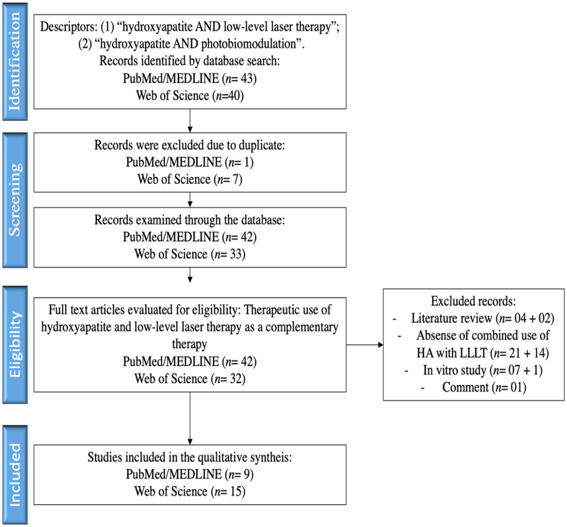
The bibliographic search, with the descriptors “hydroxyapatite AND low-level laser therapy” and “hydroxyapatite AND photobiomodulation” resulted in 43 articles in the PubMed/MEDLINE database, of which 1 was excluded for being a duplicate and another 33 due to inclusion/exclusion criteria, totaling 9 articles for qualitative analysis. In the Web of Science database, we obtained 40 articles, of which 7 were excluded for being duplicates, 1 for not having the full text available and another 17 due to inclusion/exclusion criteria, totaling 15 articles for qualitative analysis.
The most used biomaterial was composed of hydroxyapatite and β-tricalcium phosphate in a proportion of 70%–30%. In photobiomodulation, the gallium-aluminum-arsenide (GaAlAs) laser prevailed, with a wavelength of 780 nm, followed by 808 nm.
The results indicated that the use of laser phototherapy improved the repair of bone defects grafted with the biomaterial, increasing the deposition of HA phosphate as indicated by biochemical estimators, spectroscopy and histological analyses.
Citation: Jéssica de Oliveira Rossi, Gabriel Tognon Rossi, Maria Eduarda Côrtes Camargo, Rogerio Leone Buchaim, Daniela Vieira Buchaim. Effects of the association between hydroxyapatite and photobiomodulation on bone regeneration[J]. AIMS Bioengineering, 2023, 10(4): 466-490. doi: 10.3934/bioeng.2023027
Hydroxyapatite (HA)-based ceramics are widely used as artificial bone substitutes due to their advantageous biological properties, which include biocompatibility, biological affinity, bioactivity, ability to drive bone formation, integration into bone tissue and induction of bone regeneration (in certain conditions). Phototherapy in bone regeneration is a therapeutic approach that involves the use of light to stimulate and accelerate the process of repair and regeneration of bone tissue. There are two common forms of phototherapy used for this purpose: Low-Level Laser Therapy (LLLT) and LED (Light Emitting Diode) Therapy. Understanding the mechanisms of laser therapy and its effects combined with hydroxyapatite has gaps. Therefore, this review was designed based on the PICO strategy (P: problem; I: intervention; C: control; O: result) to analyze the relationship between PBM therapy and hydroxyapatite.
The bibliographic search, with the descriptors “hydroxyapatite AND low-level laser therapy” and “hydroxyapatite AND photobiomodulation” resulted in 43 articles in the PubMed/MEDLINE database, of which 1 was excluded for being a duplicate and another 33 due to inclusion/exclusion criteria, totaling 9 articles for qualitative analysis. In the Web of Science database, we obtained 40 articles, of which 7 were excluded for being duplicates, 1 for not having the full text available and another 17 due to inclusion/exclusion criteria, totaling 15 articles for qualitative analysis.
The most used biomaterial was composed of hydroxyapatite and β-tricalcium phosphate in a proportion of 70%–30%. In photobiomodulation, the gallium-aluminum-arsenide (GaAlAs) laser prevailed, with a wavelength of 780 nm, followed by 808 nm.
The results indicated that the use of laser phototherapy improved the repair of bone defects grafted with the biomaterial, increasing the deposition of HA phosphate as indicated by biochemical estimators, spectroscopy and histological analyses.

| [1] |
de Oliveira Gonçalves JB, Buchaim DV, de Souza Bueno CR, et al. (2016) Effects of low-level laser therapy on autogenous bone graft stabilized with a new heterologous fibrin sealant. J Photochem Photobiol 162: 663-668. https://doi.org/10.1016/j.jphotobiol.2016.07.023 
|
| [2] |
Magri AMP, Parisi JR, de Andrade ALM, et al. (2021) Bone substitutes and photobiomodulation in bone regeneration: A systematic review in animal experimental studies. J Biomed Mater Res A 109: 1765-1775. https://doi.org/10.1002/jbm.a.37170
|
| [3] |
Gillman CE, Jayasuriya AC (2021) FDA-approved bone grafts and bone graft substitute devices in bone regeneration. Mater Sci Eng 130: 112466. https://doi.org/10.1016/j.msec.2021.112466
|
| [4] |
Campana V, Milano G, Pagano E, et al. (2014) Bone substitutes in orthopaedic surgery: from basic science to clinical practice. J Mater Sci Mater Med 25: 2445-2461. https://doi.org/10.1007/s10856-014-5240-2
|
| [5] |
Baldwin P, Li DJ, Auston DA, et al. (2019) Autograft, allograft, and bone graft substitutes: Clinical evidence and indications for use in the setting of orthopaedic trauma surgery. J Orthop Trauma 33: 203-213. https://doi.org/10.1097/BOT.0000000000001420
|
| [6] |
Albrektsson T, Johansson C (2001) Osteoinduction, osteoconduction and osseointegration. Eur Spine J 10: S96-S101. https://doi.org/10.1007/s005860100282
|
| [7] |
Hing KA (2004) Bone repair in the twenty–first century: biology, chemistry or engineering?. Phil Trans R Soc A 362: 2821-2850. https://doi.org/10.1098/rsta.2004.1466
|
| [8] |
Campion CR, Ball SL, Clarke DL, et al. (2013) Microstructure and chemistry affects apatite nucleation on calcium phosphate bone graft substitutes. J Mater Sci Mater Med 24: 597-610. https://doi.org/10.1007/s10856-012-4833-x
|
| [9] |
Jarcho M (1981) Calcium phosphate ceramics as hard tissue prosthetics. Clin Orthop Relat Res 157: 259-278. https://doi.org/10.1097/00003086-198106000-00037
|
| [10] |
Mendelson BC, Jacobson SR, Lavoipierre AM, et al. (2010) The fate of porous hydroxyapatite granules used in facial skeletal augmentation. Aesthetic Plast Surg 34: 455-461. https://doi.org/10.1007/s00266-010-9473-2
|
| [11] |
Kattimani VS, Kondaka S, Lingamaneni KP (2016) Hydroxyapatite–past, present, and future in bone regeneration. Bone Tissue Regen Insights 7: BTRI.S36138. https://doi.org/10.4137/BTRI.S36138
|
| [12] |
Hamblin MR (2016) Photobiomodulation or low-level laser therapy. J Biophotonics 9: 1122-1124. https://doi.org/10.1002/jbio.201670113
|
| [13] |
Reis CHB, Buchaim DV, Ortiz AC, et al. (2022) Application of fibrin associated with photobiomodulation as a promising strategy to improve regeneration in tissue engineering: a systematic review. Polymers 14: 3150. https://doi.org/10.3390/polym14153150
|
| [14] |
Santos CM da C, Pimenta CA de M, Nobre MRC (2007) The PICO strategy for the research question construction and evidence search. Rev Lat Am Enfermagem 15: 508-511. https://doi.org/10.1590/s0104-11692007000300023
|
| [15] |
Moher D, Liberati A, Tetzlaff J, et al. (2009) Preferred reporting items for systematic reviews and meta-analyses: the PRISMA statement. PLoS Med 6: e1000097. https://doi.org/10.1371/journal.pmed.1000097
|
| [16] | de Carvalho FB, Aciole GTS, Aciole JMS, et al. (2011) Assessment of bone healing on tibial fractures treated with wire osteosynthesis associated or not with infrared laser light and biphasic ceramic bone graft (HATCP) and guided bone regeneration (GBR): Raman spectroscopy study. Proc. SPIE 7887, Mechanisms for Low-Light Therapy VI: 78870T 7887: 157-162. https://doi.org/10.1117/12.874288 |
| [17] |
dos Santos Aciole JM, dos Santos Aciole GT, Soares LGP, et al. (2011) Bone repair on fractures treated with osteosynthesis, ir laser, bone graft and guided bone regeneration: histomorfometric study. AIP Conference Proceedings American Institute of Physics 1364: 60-65. https://doi.org/10.1063/1.3626913
|
| [18] |
Soares LGP, Marques AMC, Guarda MG, et al. (2014) Influence of the λ780nm laser light on the repair of surgical bone defects grafted or not with biphasic synthetic micro-granular hydroxylapatite+Beta-Calcium triphosphate. J Photochem Photobiol B 131: 16-23. https://doi.org/10.1016/j.jphotobiol.2013.12.015
|
| [19] | Soares LGP, Marques AMC, Aciole JMS, et al. (2014) Assessment laser phototherapy on bone defects grafted or not with biphasic synthetic micro-granular HA + β-Tricalcium phosphate: histological study in an animal model. Proc. SPIE 8932, Mechanisms for Low-Light Therapy IX. SPIE 8932: 207-212. https://doi.org/10.1117/12.2036872 |
| [20] |
de Castro ICV, Rosa CB, dos Reis Júnior JA, et al. (2014) Assessment of the use of LED phototherapy on bone defects grafted with hydroxyapatite on rats with iron-deficiency anemia and nonanemic: a Raman spectroscopy analysis. Lasers Med Sci 29: 1607-1615. https://doi.org/10.1007/s10103-014-1562-z
|
| [21] |
Soares LGP, Marques AMC, Guarda MG, et al. (2014) Raman spectroscopic study of the repair of surgical bone defects grafted or not with biphasic synthetic micro-granular HA + β-calcium triphosphate irradiated or not with λ850 nm LED light. Lasers Med Sci 29: 1927-1936. https://doi.org/10.1007/s10103-014-1601-9
|
| [22] |
Soares LGP, Marques AMC, Barbosa AFS, et al. (2014) Raman study of the repair of surgical bone defects grafted with biphasic synthetic microgranular HA + β-calcium triphosphate and irradiated or not with λ780 nm laser. Lasers Med Sci 29: 1539-1550. https://doi.org/10.1007/s10103-013-1297-2
|
| [23] |
Pinheiro ALB, Soares LGP, Marques AMC, et al. (2017) Biochemical changes on the repair of surgical bone defects grafted with biphasic synthetic micro-granular HA + β-tricalcium phosphate induced by laser and LED phototherapies and assessed by Raman spectroscopy. Lasers Med Sci 32: 663-672. https://doi.org/10.1007/s10103-017-2165-2
|
| [24] |
Pinheiro ALB, Soares LGP, Marques AMC, et al. (2014) Raman ratios on the repair of grafted surgical bone defects irradiated or not with laser (λ780nm) or LED (λ850nm). J Photochem Photobiol B 138: 146-154. https://doi.org/10.1016/j.jphotobiol.2014.05.022
|
| [25] |
Pinheiro ALB, Aciole GTS, Ramos TA, et al. (2013) The efficacy of the use of IR laser phototherapy associated to biphasic ceramic graft and guided bone regeneration on surgical fractures treated with miniplates: a histological and histomorphometric study on rabbits. Lasers Med Sci 29: 279-288. https://doi.org/10.1007/s10103-013-1339-9
|
| [26] | Pinheiro ALB, Soares LGP, Marques AMC, et al. (2014) Raman and histological study of the repair of surgical bone defects grafted with biphasic synthetic micro-granular HA+ β-calcium triphosphate and irradiated or not with λ780 nm laser. Mechanisms for Low-Light Therapy IX. SPIE 8932: 148-155. https://doi.org/10.1117/12.2036867 |
| [27] |
Pinheiro ALB, Santos NRS, Oliveira PC, et al. (2013) The efficacy of the use of IR laser phototherapy associated to biphasic ceramic graft and guided bone regeneration on surgical fractures treated with wire osteosynthesis: a comparative laser fluorescence and Raman spectral study on rabbits. Lasers Med Sci 28: 815-822. https://doi.org/10.1007/s10103-012-1166-4
|
| [28] |
Soares LGP, Marques AMC, Aciole JMS, et al. (2014) Do laser/LED phototherapies influence the outcome of the repair of surgical bone defects grafted with biphasic synthetic microgranular HA + β-tricalcium phosphate? A Raman spectroscopy study. Lasers Med Sci 29: 1575-1584. https://doi.org/10.1007/s10103-014-1563-y
|
| [29] | Soares LGGP, Aciole JMS, Aciole GTS, et al. (2013) Raman study of the effect of LED light on grafted bone defects. Proc. SPIE 8569, Mechanisms for Low-Light Therapy VIII. SPIE 8569: 102-109. https://doi.org/10.1117/12.2002584 |
| [30] |
Pinheiro ALB, Santos NRS, Oliveira PC, et al. (2013) The efficacy of the use of IR laser phototherapy associated to biphasic ceramic graft and guided bone regeneration on surgical fractures treated with miniplates: a Raman spectral study on rabbits. Lasers Med Sci 28: 513-518. https://doi.org/10.1007/s10103-012-1096-1
|
| [31] |
Reis CHB, Buchaim RL, Pomini KT, et al. (2022) Effects of a Biocomplex Formed by Two Scaffold Biomaterials, Hydroxyapatite/Tricalcium Phosphate Ceramic and Fibrin Biopolymer, with Photobiomodulation, on Bone Repair. Polymers 14: 2075. https://doi.org/10.3390/polym14102075
|
| [32] |
de Oliveira GJPL, Pinotti FE, Aroni MAT, et al. (2021) Effect of different low-level intensity laser therapy (LLLT) irradiation protocols on the osseointegration of implants placed in grafted areas. J Appl Oral Sci 29: e20200647. https://doi.org/10.1590/1678-7757-2020-0647
|
| [33] |
de Oliveira GJPL, Aroni MAT, Pinotti FE, et al. (2020) Low-level laser therapy (LLLT) in sites grafted with osteoconductive bone substitutes improves osseointegration. Lasers Med Sci 35: 1519-1529. https://doi.org/10.1007/s10103-019-02943-w
|
| [34] |
Theodoro LH, Rocha GS, Ribeiro Junior VL, et al. (2018) Bone formed after maxillary sinus floor augmentation by bone autografting with hydroxyapatite and low-level laser therapy: A randomized controlled trial with histomorphometrical and immunohistochemical analyses. Implant Dent 27: 547-554. https://doi.org/10.1097/ID.0000000000000801
|
| [35] |
de Oliveira GJPL, Aroni MAT, Medeiros MC, et al. (2018) Effect of low-level laser therapy on the healing of sites grafted with coagulum, deproteinized bovine bone, and biphasic ceramic made of hydroxyapatite and β-tricalcium phosphate. In vivo study in rats. Lasers Surg Med 50: 651-660. https://doi.org/10.1002/lsm.22787
|
| [36] |
Alan H, Vardi N, Özgür C, et al. (2015) Comparison of the Effects of Low-Level Laser Therapy and Ozone Therapy on Bone Healing. J Craniofac Surg 26: e396-e400. https://doi.org/10.1097/SCS.0000000000001871
|
| [37] |
Pinheiro ALB, Martinez Gerbi ME, de Assis Limeira F, et al. (2009) Bone repair following bone grafting hydroxyapatite guided bone regeneration and infra-red laser photobiomodulation: a histological study in a rodent model. Lasers Med Sci 24: 234-240. https://doi.org/10.1007/s10103-008-0556-0
|
| [38] |
Dalapria V, Marcos RL, Bussadori SK, et al. (2022) LED photobiomodulation therapy combined with biomaterial as a scaffold promotes better bone quality in the dental alveolus in an experimental extraction model. Lasers Med Sci 37: 1583-1592. https://doi.org/10.1007/s10103-021-03407-w
|
| [39] |
Franco GR, Laraia IO, Maciel AAW, et al. (2013) Effects of chronic passive smoking on the regeneration of rat femoral defects filled with hydroxyapatite and stimulated by laser therapy. Injury 44: 908-913. https://doi.org/10.1016/j.injury.2012.12.022
|
| [40] |
Pomini KT, Cestari TM, Santos German ÍJ, et al. (2019) Influence of experimental alcoholism on the repair process of bone defects filled with beta-tricalcium phosphate. Drug Alcohol Depend 197: 315-325. https://doi.org/10.1016/j.drugalcdep.2018.12.031
|
| [41] | Tanishka T, Anjali B, Shefali M, et al. (2023) An insight into the biomaterials used in craniofacial tissue engineering inclusive of regenerative dentistry. AIMS Bioengineering 10: 153-174. https://doi.org/10.3934/bioeng.2023011 |
| [42] | Jing X, Ding Q, Wu Q, et al. (2021) Magnesium-based materials in orthopaedics: material properties and animal models. Biomater Transl 2: 197-213. https://doi.org/10.12336/biomatertransl.2021.03.004 |
| [43] | Steijvers E, Ghei A, Xia Z (2022) Manufacturing artificial bone allografts: a perspective. Biomater Transl 3: 65-80. https://doi.org/10.12336/biomatertransl.2022.01.007 |
| [44] | Tai A, Landao-Bassonga E, Chen Z, et al. (2023) Systematic evaluation of three porcine-derived collagen membranes for guided bone regeneration. Biomater Transl 4: 41-50. https://doi.org/10.12336/biomatertransl.2023.01.006 |
| [45] |
Della Coletta BB, Jacob TB, Moreira LAC, et al. (2021) Photobiomodulation therapy on the guided bone regeneration process in defects filled by biphasic calcium phosphate associated with fibrin biopolymer. Molecules 26: 847. https://doi.org/10.3390/molecules26040847
|
| [46] |
Ono N (2022) The mechanism of bone repair: Stem cells in the periosteum dedicated to bridging a large gap. Cell Rep Med 3: 100807. https://doi.org/10.1016/j.xcrm.2022.100807
|
| [47] |
Wang Y, Zhang H, Hu Y, et al. (2022) Bone repair biomaterials: a perspective from immunomodulation. Adv Funct Mater 32: 2208639. https://doi.org/10.1002/adfm.202208639
|
| [48] |
Han L, Mengmeng L, Tao Z, et al. (2022) Engineered bacterial extracellular vesicles for osteoporosis therapy. Chem Eng J 450: 138309. https://doi.org/10.1016/j.cej.2022.138309
|
| [49] |
de Moraes R, Plepis AMdG, Martins VdCA, et al. (2023) Viability of collagen matrix grafts associated with nanohydroxyapatite and elastin in bone repair in the experimental condition of ovariectomy. Int J Mol Sci 24: 15727. https://doi.org/10.3390/ijms242115727
|


Figures(3) / Tables(1)

Jéssica de Oliveira Rossi, Gabriel Tognon Rossi, Maria Eduarda Côrtes Camargo, Rogerio Leone Buchaim, Daniela Vieira Buchaim. Effects of the association between hydroxyapatite and photobiomodulation on bone regeneration[J]. AIMS Bioengineering, 2023, 10(4): 466-490. doi: 10.3934/bioeng.2023027


 DownLoad: