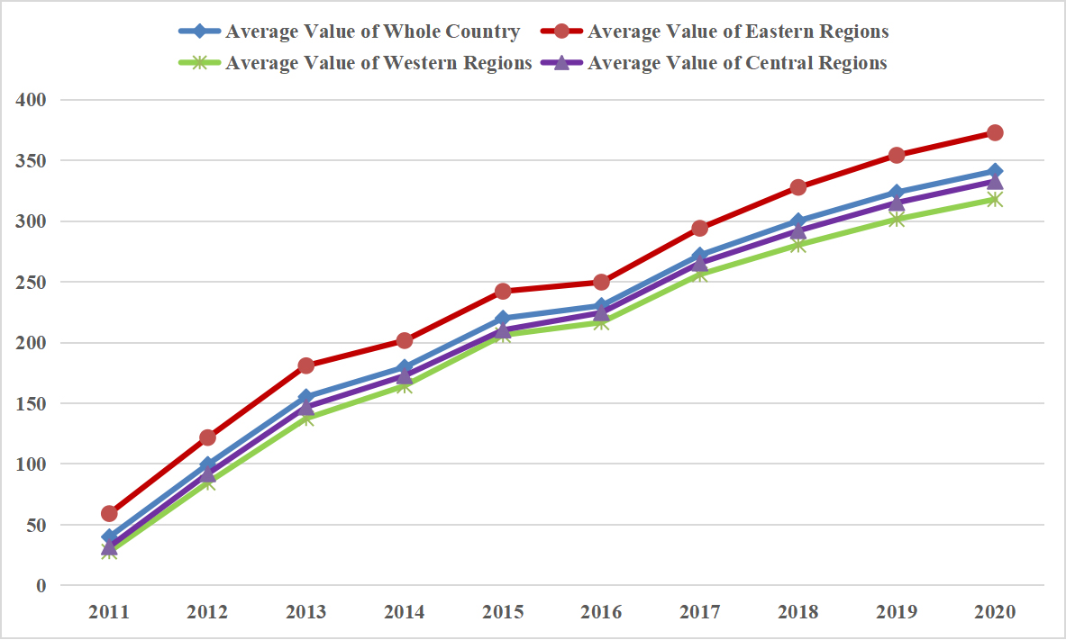
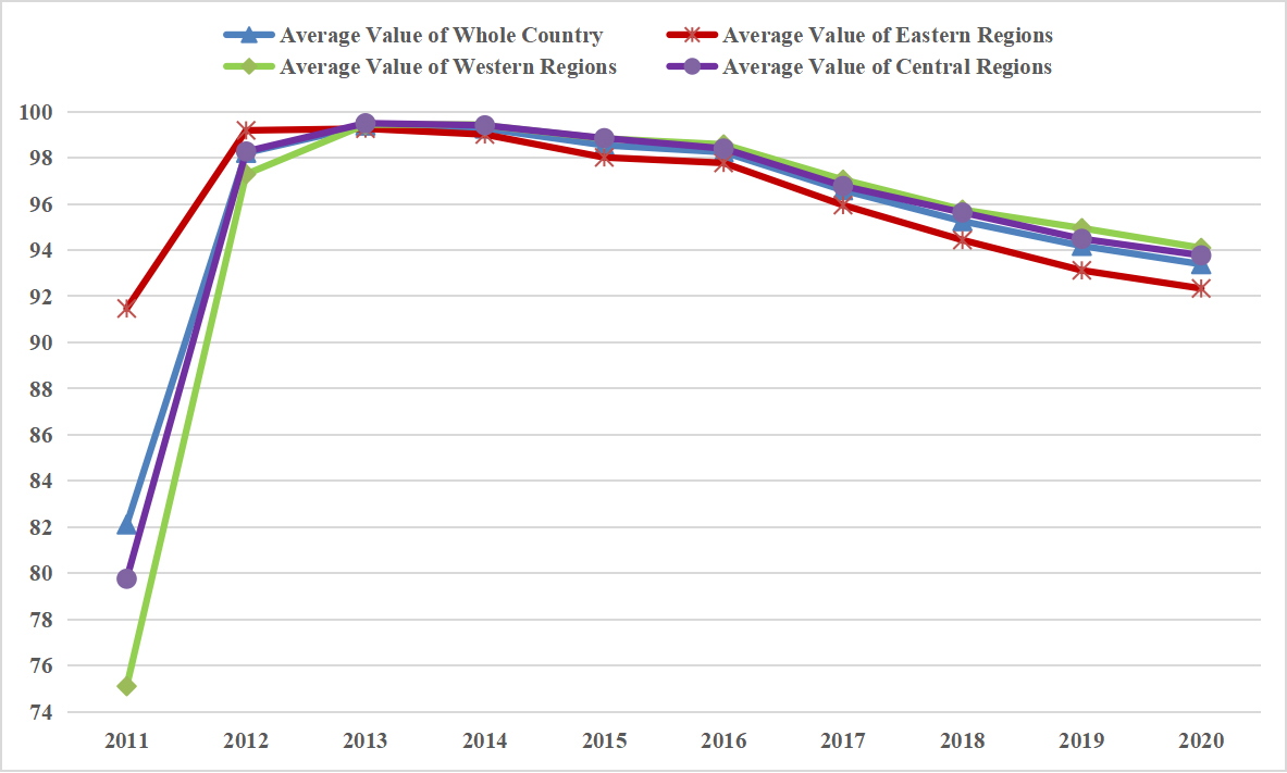
Effective development of digital finance is vital to closing the regional economic disparities. This study aims at investigating the efficiency of digital finance development in China and its implications for closing regional economic disparities. Using the stochastic frontier model, we estimate the development efficiency of digital finance in 31 provinces in China from 2011 to 2020, and reveal their characteristics of temporal evolution and spatial distribution. The results show that the efficiency of digital finance development in each province shows a tendency to increase quickly first and then slowly decline. The provinces with a higher level of digital finance development always have higher development efficiency at the beginning of the sample period, which then declines rapidly after reaching the maximum, and even less than the national average value at the end of the period, with significant regional disparities observed. The provinces with a higher level of digital finance development always have higher development efficiency at the beginning of the sample period, which then declines rapidly after reaching the maximum, and even less than the national average value at the end of the period. The imbalance of development efficiency among different provinces is increasing, and the potential for development efficiency in the central and western regions is relatively greater. These findings have important implications for promoting high-quality economic development and common prosperity in China. In the future, we should continually prevent the development efficiency of digital finance to decline rapidly in all provinces (especially in the eastern region), and strive constantly to bridge the gap of development efficiency among different province, so as to provide a better surrounding for promoting high-quality economic development and common prosperity.
Citation: Guang Liu, Hong Yi, Haonan Liang. Measuring provincial digital finance development efficiency based on stochastic frontier model[J]. Quantitative Finance and Economics, 2023, 7(3): 420-439. doi: 10.3934/QFE.2023021
Effective development of digital finance is vital to closing the regional economic disparities. This study aims at investigating the efficiency of digital finance development in China and its implications for closing regional economic disparities. Using the stochastic frontier model, we estimate the development efficiency of digital finance in 31 provinces in China from 2011 to 2020, and reveal their characteristics of temporal evolution and spatial distribution. The results show that the efficiency of digital finance development in each province shows a tendency to increase quickly first and then slowly decline. The provinces with a higher level of digital finance development always have higher development efficiency at the beginning of the sample period, which then declines rapidly after reaching the maximum, and even less than the national average value at the end of the period, with significant regional disparities observed. The provinces with a higher level of digital finance development always have higher development efficiency at the beginning of the sample period, which then declines rapidly after reaching the maximum, and even less than the national average value at the end of the period. The imbalance of development efficiency among different provinces is increasing, and the potential for development efficiency in the central and western regions is relatively greater. These findings have important implications for promoting high-quality economic development and common prosperity in China. In the future, we should continually prevent the development efficiency of digital finance to decline rapidly in all provinces (especially in the eastern region), and strive constantly to bridge the gap of development efficiency among different province, so as to provide a better surrounding for promoting high-quality economic development and common prosperity.

| [1] |
Aigner D, Lovell C, Schmidt P (1977) Formulation and estimation of stochastic frontier production function models. J Econometrics 6: 21–37. https://doi.org/10.1016/0304-4076(77)90052-5 doi: 10.1016/0304-4076(77)90052-5

|
| [2] | Aigner DJ, Chu SF (1968) On estimating the industry production function. Am Econ Rev 58: 826–839. http://www.jstor.org/stable/1815535 |
| [3] | Bai JH, Jiang KS, Li J (2009) Exploiting the model of the stochastic frontier to measure and evaluate the efficiency of the regional R & D innovation in China. Manage World 10: 51–61. |
| [4] |
Banker R, Cooper WW (1984) Some models for estimating technical and scale inefficiencies in data envelopment analysis. Manage Sci 30: 1078–1092. https://doi.org/10.1287/mnsc.30.9.1078 doi: 10.1287/mnsc.30.9.1078
|
| [5] | Banks E (2001) e-Finance: the electronic revolution in financial services, In: Banks E, 1 Edn., New York: John Wiley and Sons Press, Inc. |
| [6] |
Barbesino P, Camerani R, Gaudino A (2005) Digital finance in Europe: Competitive dynamics and online behaviour. J Financ Serv Mark 94: 329–343. https://doi.org/10.1057/palgrave.fsm.4770164 doi: 10.1057/palgrave.fsm.4770164
|
| [7] |
Battese GE, Coelli TJ (1995) A model for technical inefficiency effects in a stochastic frontier production function for panel data. Empir Econ 20: 325–332. https://doi.org/10.1007/BF01205442 doi: 10.1007/BF01205442
|
| [8] |
Charnes AW, Cooper WW, Rhodes EL (1979) Measuring the inefficiency of decision making units. European Journal of Operational Research 3: 339–338. https://doi.org/10.1016/0377-2217(79)90229-7 doi: 10.1016/0377-2217(79)90229-7
|
| [9] |
Chen K-H, Ghosh SN (2014) Threshold effects of technological regimes for the stochastic frontier model. J Dev Areas. https://doi.org/10.1353/jda.2014.0040 doi: 10.1353/jda.2014.0040
|
| [10] |
Christensen LR, Jorgenson DW, Lau LJ (1973) Transcendental logarithmic production frontiers. Rev Econ Stat 55: 28–45. https://doi.org/10.2307/1927992 doi: 10.2307/1927992
|
| [11] |
Cornwell C, Schmidt P (1996) Production frontiers and efficiency measurement. The econometrics of panel data: a handbook of the theory with applications. https://doi.org/10.1007/978-94-009-0137-7_33 doi: 10.1007/978-94-009-0137-7_33
|
| [12] |
Debreu G. (1951) The coefficient of resource utilization. Econometrica 19: 273–292. https://doi.org/10.2307/1906814 doi: 10.2307/1906814
|
| [13] | Fare R, Grosskopf S, Lovell CAK (1985) The Measurement of Efficiency of Production[M]. Springer Sci Bus Media 6. https://doi.org/10.1007/978-94-015-7721-2 |
| [14] |
Fare R, Lovell CAK (1978) Measuring the technical efficiency of production. J Econ Theory 19: 150–162. https://doi.org/10.1016/0022-0531(78)90060-1 doi: 10.1016/0022-0531(78)90060-1
|
| [15] |
Farrell JM (1957) The measurement of productive efficiency. J Royal Stat Society 120: 253–290. https://doi.org/10.2307/2343100 doi: 10.2307/2343100
|
| [16] | Fu QZ, Huang YP (2018) Digital finance's heterogeneous effects on rural financial demand: Evidence from China household finance survey and inclusive digital finance index. J Financ Res 11: 68–84. |
| [17] |
Gong BH, Sickles RC (1992) Finite sample evidence on the performance of stochastic frontiers and data envelopment analysis using panel data. J Econometrics 51: 259–284. https://doi.org/10.1016/0304-4076(92)90038-S doi: 10.1016/0304-4076(92)90038-S
|
| [18] | Greene WH (2008) The econometric approach to efficiency analysis, In: Harold O. Fried, C. A. Knox Lovell and S. S. Schmidt Greene W H, The measurement of productive efficiency productivity growth, New York: Oxford University Press, 92–250. https://doi.org/10.1093/acprof: oso/9780195183528.003.0002 |
| [19] | Guo F, Wang JY, Wang F, et al. (2020) Measuring China's digital financial inclusion: Index compilation and spatial characteristics. China Econ Q 19: 1401–1418. |
| [20] |
Jondrow J, Lovell CAK, Materov IS, et al. (1982) On the estimation of technical inefficiency in the stochastic frontier production function model. J Econometrics 19: 233–238. https://doi.org/10.1016/0304-4076(82)90004-5 doi: 10.1016/0304-4076(82)90004-5
|
| [21] | Koopmans T (1951) An analysis of Production as an Efficient Combination of Activities. In: Activity Analysis of Production and Allocation, New York: John Wiley and Sons Press, Vol.13 of Cowles Commission for Research in Economics: 33–97. https://cir.nii.ac.jp/crid/1572824499992043008 |
| [22] | Kumbhakar SC, Lovell CK (2003) Stochastic frontier analysis, In: Kumbhakar SC, Lovell CK, Cambridge University Press. |
| [23] |
Lee S, Lee YH (2014) Stochastic frontier models with threshold efficiency. J Prod Anal, 4245–4254. https://doi.org/10.1007/s11123-013-0364-9 doi: 10.1007/s11123-013-0364-9
|
| [24] |
Liao GK, Li ZH, Wang MX, et al. (2022) Measuring China's urban digital finance. Quant Financ Econ 6: 385–404. https://doi.org/10.3934/QFE.2022017 doi: 10.3934/QFE.2022017
|
| [25] | Manyika J, Lund S, singer M, et al. (2016) Digital finance for all: Powering inclusive growth in emerging economies. McKinsey Global Institute, 1–5. |
| [26] |
Mastromarco C, Serlenga L, Shin Y (2012) Is globalization driving efficiency? A threshold stochastic frontier panel data modeling approach. Rev Int Econ 203: 563–579. https://doi.org/10.1111/j.1467-9396.2012.01039.x doi: 10.1111/j.1467-9396.2012.01039.x
|
| [27] |
Meeusen W, van Den Broeck J (1977) Efficiency estimation from Cobb-Douglas production functions with composed error. Int Econ Rev 18: 435–444. https://doi.org/10.2307/2525757 doi: 10.2307/2525757
|
| [28] |
Ondrich J, Ruggiero J (2001) Efficiency measurement in the stochastic frontier model. Eur J Oper Res 129: 434–442. https://doi.org/10.1016/S0377-2217(99)00429-4 doi: 10.1016/S0377-2217(99)00429-4
|
| [29] |
Ozili PK (2018) Impact of digital finance on financial inclusion and stability. Borsa Istanbul Rev 184: 329–340. https://doi.org/10.1016/j.bir.2017.12.003. doi: 10.1016/j.bir.2017.12.003
|
| [30] | Rizzo M (2014) Digital finance: Empowering the poor via new technologies. Washington DC: The Word Bank. Available from: https://www.worldbank.org/en/news/feature/2014/04/10/digital-finance-empowering-poor-new-technologies. |
| [31] |
Scott SV, Van Reenen J, Zachariadis M (2017) The long-term effect of digital innovation on bank performance: An empirical study of SWIFT adoption in financial services. Res Policy 465: 984–1004. https://doi.org/10.1016/j.respol.2017.03.010 doi: 10.1016/j.respol.2017.03.010
|
| [32] |
Tsionas EG, Tran KC, Michaelides PG (2019) Bayesian inference in threshold stochastic frontier models. Empir Econ, 56399–56422. https://doi.org/10.1007/s00181-017-1364-9 doi: 10.1007/s00181-017-1364-9
|
| [33] |
Yao L, Ma X (2022) Has digital finance widened the income gap? Plos one 172: e0263915. https://doi.org/10.1371/journal.pone.0263915 doi: 10.1371/journal.pone.0263915
|
| [34] | Zhang JY, Hu ZM (2022) Spatiotemporal characteristics and influencing factors of China's urban digital inclusive finance development. J Southwest Minzu University (Humanities and Social Science) 43: 108–118. |
| [35] | Zhang LY, Xing CH (2021) Distribution dynamics, regional differences and convergence of digital inclusive finance in rural China. J Quant Technical Econ 38: 23–42. |
| [36] | Zhang YT, Yang L (2020) National financial development of the "Belt and Road" countries and efficiency of China's foreign direct investment. J Quant Technical Econ 37: 109–124. |
Figures(2) / Tables(10)

Guang Liu, Hong Yi, Haonan Liang. Measuring provincial digital finance development efficiency based on stochastic frontier model[J]. Quantitative Finance and Economics, 2023, 7(3): 420-439. doi: 10.3934/QFE.2023021


 DownLoad: