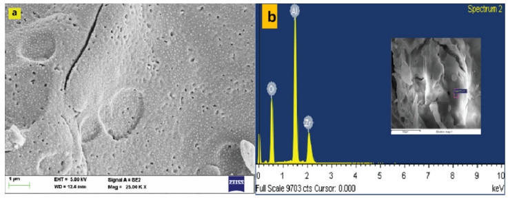
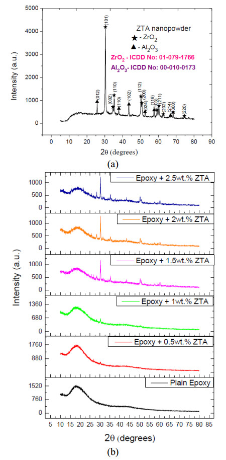
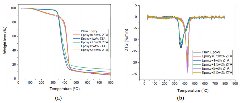
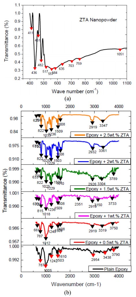
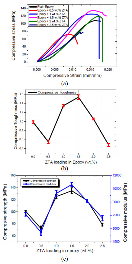
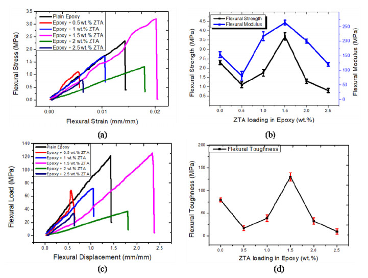
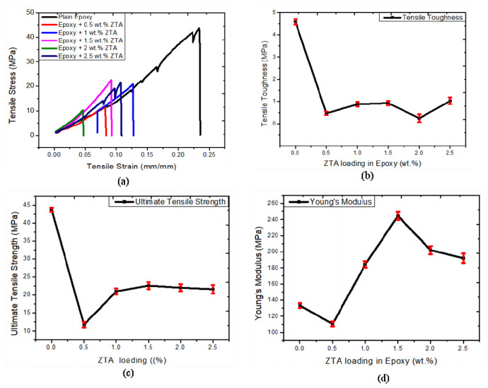
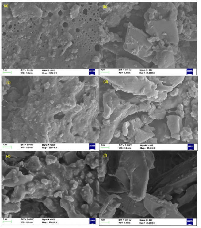
Epoxy composites were prepared by doping nano Zirconia Toughened Alumina (ZTA) which were synthesized by solution combustion method into epoxy resin and hardener. Initially ZTA nanopowder was characterized to check its purity, morphology and to confirm its metal-oxide bonding using XRD, SEM and FTIR respectively. The thermal properties such as TGA and DTG were also analysed. The polymer composites were obtained by uniformly dispersing ZTA nanopowder into epoxy using an ultrasonicator. Polymer composites of various concentrations viz, 0.5, 1, 1.5, 2 and 2.5 wt% were synthesized, all concentrations were prepared on weight basis. All the polymer composites were tested for compression properties, flexural properties and tensile properties. Best results for all the mechanical properties were obtained for epoxy with 1.5 wt% ZTA composites. Electrical properties such as breakdown voltage and breakdown strength were analysed and outstanding results were observed for epoxy with 2.5 wt% ZTA composite.
Citation: Chaitra Srikanth, G.M. Madhu, Shreyas J. Kashyap. Enhanced structural, thermal, mechanical and electrical properties of nano ZTA/epoxy composites[J]. AIMS Materials Science, 2022, 9(2): 214-235. doi: 10.3934/matersci.2022013
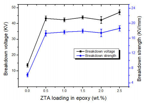
Epoxy composites were prepared by doping nano Zirconia Toughened Alumina (ZTA) which were synthesized by solution combustion method into epoxy resin and hardener. Initially ZTA nanopowder was characterized to check its purity, morphology and to confirm its metal-oxide bonding using XRD, SEM and FTIR respectively. The thermal properties such as TGA and DTG were also analysed. The polymer composites were obtained by uniformly dispersing ZTA nanopowder into epoxy using an ultrasonicator. Polymer composites of various concentrations viz, 0.5, 1, 1.5, 2 and 2.5 wt% were synthesized, all concentrations were prepared on weight basis. All the polymer composites were tested for compression properties, flexural properties and tensile properties. Best results for all the mechanical properties were obtained for epoxy with 1.5 wt% ZTA composites. Electrical properties such as breakdown voltage and breakdown strength were analysed and outstanding results were observed for epoxy with 2.5 wt% ZTA composite.

| [1] |
Wetzel B, Haupert F, Zhang MQ (2003) Epoxy nanocomposites with high mechanical and tribological performance. Compos Sci Technol 63: 2055-2067. https://doi.org/10.1016/S0266-3538(03)00115-5 doi: 10.1016/S0266-3538(03)00115-5

|
| [2] |
Carolan D, Ivankovic A, Kinloch AJ, et al. (2017) Toughened carbon fibre-reinforced polymer composites with nanoparticle-modified epoxy matrices. J Mater Sci 52: 1767-1788. https://doi.org/10.1007/s10853-016-0468-5 doi: 10.1007/s10853-016-0468-5
|
| [3] |
Dorigato A, Pegoretti A, Bondioli F, et al. (2010) Improving epoxy adhesives with zirconia nanoparticles. Compos Interface 17: 873-892. https://doi.org/10.1163/092764410X539253 doi: 10.1163/092764410X539253
|
| [4] |
Bondioli F, Cannillo V, Fabbri E, et al. (2006) Preparation and characterization of epoxy resins filled with submicron spherical zirconia particles. Polimery 51: 794-798. https://doi.org/10.14314/polimery.2006.794 doi: 10.14314/polimery.2006.794
|
| [5] |
Dorigato A, Pegoretti A (2011) The role of alumina nanoparticles in epoxy adhesives. J Nanopart Res 13: 2429-2441. https://doi.org/10.1007/s11051-010-0130-0 doi: 10.1007/s11051-010-0130-0
|
| [6] |
Yu ZQ, You SL, Yang ZG, et al. (2011) Effect of surface functional modification of nano-alumina particles on thermal and mechanical properties of epoxy nanocomposites. Adv Compos Mater 20: 487-502. https://doi.org/10.1163/092430411X579104 doi: 10.1163/092430411X579104
|
| [7] |
Reyes-Rojas A, Dominguez-Rios C, Garcia-Reyes A, et al. (2018) Sintering of carbon nanotube-reinforced zirconia-toughened alumina composites prepared by uniaxial pressing and cold isostatic pressing. Mater Res Express 5: 105602. https://doi.org/10.1088/2053-1591/aada35 doi: 10.1088/2053-1591/aada35
|
| [8] | Chuankrerkkul N, Somton K, Wonglom T, et al. (2016) Physical and mechanical properties of zirconia toughened alumina (ZTA) composites fabricated by powder injection moulding. Chiang Mai J Sci 43: 375-380. |
| [9] |
Ponnilavan V, Kannan S (2019) Structural, optical tuning, and mechanical behavior of zirconia toughened alumina through europium substitutions. J Biomed Mater Res Part B 107: 1170-1179. https://doi.org/10.1002/jbm.b.34210 doi: 10.1002/jbm.b.34210
|
| [10] |
Srikanth C, Madhu GM (2020) Effect of ZTA concentration on structural, thermal, mechanical and dielectric behavior of novel ZTA-PVA nanocomposite films. SN Appl Sci 2: 1-12. https://doi.org/10.1007/s42452-020-2232-3 doi: 10.1007/s42452-020-2232-3
|
| [11] |
Zhang J, Ge L, Chen ZG, et al. (2019) Cracking behavior and mechanism of gibbsite crystallites during calcination. Cryst Res Technol 54: 1800201. https://doi.org/10.1002/crat.201800201 doi: 10.1002/crat.201800201
|
| [12] |
Bhaduri S, Bhaduri SB, Zhou E (1998) Auto ignition synthesis and consolidation of Al2O3-ZrO2 nano/nano composite powders. J Mater Res 13: 156-165. https://doi.org/10.1557/JMR.1998.0021 doi: 10.1557/JMR.1998.0021
|
| [13] |
Vasylkiv O, Sakka Y, Skorokhod VV (2003) Low-temperature processing and mechanical properties of zirconia and zirconia-alumina nanoceramics. J Am Ceram Soc 86: 299-304. https://doi.org/10.1111/j.1151-2916.2003.tb00015.x doi: 10.1111/j.1151-2916.2003.tb00015.x
|
| [14] |
Sagar JS, Kashyap SJ, Madhu GM, et al. (2020) Investigation of mechanical, thermal and electrical parameters of gel combustion-derived cubic zirconia/epoxy resin composites for high-voltage insulation. Cerâmica 66: 186-196. https://doi.org/10.1590/0366-69132020663782887 doi: 10.1590/0366-69132020663782887
|
| [15] |
Ho MW, Lam CK, Lau K, et al. (2006) Mechanical properties of epoxy-based composites using nanoclays. Compos Struct 75: 415-421. https://doi.org/10.1016/j.compstruct.2006.04.051 doi: 10.1016/j.compstruct.2006.04.051
|
| [16] |
Uhl FM, Davuluri SP, Wong SC, et al. (2004) Organically modified montmorillonites in UV curable urethane acrylate films. Polymer 45: 6175-6187. https://doi.org/10.1016/j.polymer.2004.07.001 doi: 10.1016/j.polymer.2004.07.001
|
| [17] |
Nguyen TA, Nguyen TV, Thai H, et al. (2016) Effect of nanoparticles on the thermal and mechanical properties of epoxy coatings. J Nanosci Nanotechnol 16: 9874-9881. https://doi.org/10.1166/jnn.2016.12162 doi: 10.1166/jnn.2016.12162
|
| [18] |
Baiquni M, Soegijono B, Hakim AN (2019) Thermal and mechanical properties of hybrid organoclay/rockwool fiber reinforced epoxy composites. J Phys Conf Ser 1191: 012056. https://doi.org/10.1088/1742-6596/1191/1/012056 doi: 10.1088/1742-6596/1191/1/012056
|
| [19] |
Zhang X, Alloul O, He Q, et al. (2013) Strengthened magnetic epoxy nanocomposites with protruding nanoparticles on the graphene nanosheets. Polymer 54: 3594-3604. https://doi.org/10.1016/j.polymer.2013.04.062 doi: 10.1016/j.polymer.2013.04.062
|
| [20] |
Nazarenko OB, Melnikova TV, Visakh PM (2016) Thermal and mechanical characteristics of polymer composites based on epoxy resin, aluminium nanopowders and boric acid. J Phys Conf Ser 671: 012040. https://doi.org/10.1088/1742-6596/671/1/012040 doi: 10.1088/1742-6596/671/1/012040
|
| [21] |
Sand Chee S, Jawaid M (2019) The effect of Bi-functionalized MMT on morphology, thermal stability, dynamic mechanical, and tensile properties of epoxy/organoclay nanocomposites. Polymers 11: 2012. https://doi.org/10.3390/polym11122012 doi: 10.3390/polym11122012
|
| [22] |
Bikiaris D (2011) Can nanoparticles really enhance thermal stability of polymers? Part Ⅱ: An overview on thermal decomposition of polycondensation polymers. Thermochim Acta 523: 25-45. https://doi.org/10.1016/j.tca.2011.06.012 doi: 10.1016/j.tca.2011.06.012
|
| [23] |
Xue Y, Shen M, Zeng S, et al. (2019) A novel strategy for enhancing the flame resistance, dynamic mechanical and the thermal degradation properties of epoxy nanocomposites. Mater Res Express 6: 125003. https://doi.org/10.1088/2053-1591/ab537f doi: 10.1088/2053-1591/ab537f
|
| [24] |
Colomban P (1989) Structure of oxide gels and glasses by infrared and Raman scattering. J Mater Sci 24: 3011-3020. https://doi.org/10.1007/BF02385660 doi: 10.1007/BF02385660
|
| [25] |
Taavoni-Gilan A, Taheri-Nassaj E, Naghizadeh R, et al. (2010) Properties of sol-gel derived Al2O3-15 wt% ZrO2 (3 mol% Y2O3) nanopowders using two different precursors. Ceram Int 36: 1147-1153. https://doi.org/10.1016/j.ceramint.2009.11.011 doi: 10.1016/j.ceramint.2009.11.011
|
| [26] |
Noma T, Sawaoka A (1984) Fracture toughness of high pressure sintered Al2O3-ZrO2 ceramics. J Mater Sci Lett 3: 533-535. https://doi.org/10.1007/BF00720992 doi: 10.1007/BF00720992
|
| [27] |
Shukla DK, Kasisomayajula SV, Parameswaran V (2008) Epoxy composites using functionalized alumina platelets as reinforcements. Compos Sci Technol 68: 3055-3063. https://doi.org/10.1016/j.compscitech.2008.06.025 doi: 10.1016/j.compscitech.2008.06.025
|
| [28] |
Abbate M, Martuscelli E, Musto P, et al. (1994) Toughening of a highly cross-linked epoxy resin by reactive blending with bisphenol A polycarbonate. I. FTIR spectroscopy. J Polym Sci Pol Phys 32: 395-408. https://doi.org/10.1002/polb.1994.090320301 doi: 10.1002/polb.1994.090320301
|
| [29] |
Katon JE, Bentley FF (1963) New spectra-structure correlations of ketones in the 700-750 cm-1 region. Spectrochim Acta 19: 639-653. https://doi.org/10.1016/0371-1951(63)80127-7 doi: 10.1016/0371-1951(63)80127-7
|
| [30] |
Magnani G, Brillante A (2005) Effect of the composition and sintering process on mechanical properties and residual stresses in zirconia-alumina composites. J Eur Ceram Soc 25: 3383-3392. https://doi.org/10.1016/j.jeurceramsoc.2004.09.025 doi: 10.1016/j.jeurceramsoc.2004.09.025
|
| [31] |
Ashamol A, Priyambika VS, Avadhani GS, et al. (2013) Nanocomposites of crosslinked starch phthalate and silane modified nanoclay: Study of mechanical, thermal, morphological, and biodegradable characteristics. Starch-Stärke 65: 443-452. https://doi.org/10.1002/star.201200145 doi: 10.1002/star.201200145
|
| [32] |
Jumahat A, Soutis C, Mahmud J, et al. (2012) Compressive properties of nanoclay/epoxy nanocomposites. Procedia Eng 41: 1607-1613. https://doi.org/10.1016/j.proeng.2012.07.361 doi: 10.1016/j.proeng.2012.07.361
|
| [33] |
Abbass A, Abid S, Özakça M (2019) Experimental investigation on the effect of steel fibers on the flexural behavior and ductility of high-strength concrete hollow beams. Adv Civ Eng 2019: 8390345. https://doi.org/10.1155/2019/8390345 doi: 10.1155/2019/8390345
|
| [34] |
Konnola R, Deeraj BDS, Sampath S, et al. (2019) Fabrication and characterization of toughened nanocomposites based on TiO2 nanowire-epoxy system. Polym Compos 40: 2629-2638. https://doi.org/10.1002/pc.25058 doi: 10.1002/pc.25058
|
| [35] |
Zhao S, Schadler LS, Duncan R, et al. (2008) Mechanisms leading to improved mechanical performance in nanoscale alumina filled epoxy. Compos Sci Technol 68: 2965-2975. https://doi.org/10.1016/j.compscitech.2008.01.009 doi: 10.1016/j.compscitech.2008.01.009
|
| [36] |
Goyat MS, Rana S, Halder S, et al. (2018) Facile fabrication of epoxy-TiO2 nanocomposites: a critical analysis of TiO2 impact on mechanical properties and toughening mechanisms. Ultrason Sonochem 40: 861-873. https://doi.org/10.1016/j.ultsonch.2017.07.040 doi: 10.1016/j.ultsonch.2017.07.040
|
| [37] |
Johnsen BB, Kinloch AJ, Mohammed RD, et al. (2007) Toughening mechanisms of nanoparticle-modified epoxy polymers. Polymer 48: 530-541. https://doi.org/10.1016/j.polymer.2006.11.038 doi: 10.1016/j.polymer.2006.11.038
|
| [38] |
Johnsen BB, Kinloch AJ, Taylor AC (2005) Toughness of syndiotactic polystyrene/epoxy polymer blends: microstructure and toughening mechanisms. Polymer 46: 7352-7369. https://doi.org/10.1016/j.polymer.2005.05.151 doi: 10.1016/j.polymer.2005.05.151
|
| [39] |
Mohanty A, Srivastava VK (2013) Dielectric breakdown performance of alumina/epoxy resin nanocomposites under high voltage application. Mater Design 47: 711-716. https://doi.org/10.1016/j.matdes.2012.12.052 doi: 10.1016/j.matdes.2012.12.052
|
 matersci-09-02-013-s001.pdf matersci-09-02-013-s001.pdf |
 |
Figures(9) / Tables(6)

Chaitra Srikanth, G.M. Madhu, Shreyas J. Kashyap. Enhanced structural, thermal, mechanical and electrical properties of nano ZTA/epoxy composites[J]. AIMS Materials Science, 2022, 9(2): 214-235. doi: 10.3934/matersci.2022013


 DownLoad: