This article focuses on the application of deep learning and spectral analysis to epidemiology time series data, which has recently piqued the interest of some researchers. The COVID-19 virus is still mutating, particularly the delta and omicron variants, which are known for their high level of contagiousness, but policymakers and governments are resolute in combating the pandemic's spread through a recent massive vaccination campaign of their population. We used extreme machine learning (ELM), multilayer perceptron (MLP), long short-term neural network (LSTM), gated recurrent unit (GRU), convolution neural network (CNN) and deep neural network (DNN) methods on time series data from the start of the pandemic in France, Russia, Turkey, India, United states of America (USA), Brazil and United Kingdom (UK) until September 3, 2021 to predict the daily new cases and daily deaths at different waves of the pandemic in countries considered while using root mean square error (RMSE) and relative root mean square error (rRMSE) to measure the performance of these methods. We used the spectral analysis method to convert time (days) to frequency in order to analyze the peaks of frequency and periodicity of the time series data. We also forecasted the future pandemic evolution by using ELM, MLP, and spectral analysis. Moreover, MLP achieved best performance for both daily new cases and deaths based on the evaluation metrics used. Furthermore, we discovered that errors for daily deaths are much lower than those for daily new cases. While the performance of models varies, prediction and forecasting during the period of vaccination and recent cases confirm the pandemic's prevalence level in the countries under consideration. Finally, some of the peaks observed in the time series data correspond with the proven pattern of weekly peaks that is unique to the COVID-19 time series data.
Citation: Kayode Oshinubi, Augustina Amakor, Olumuyiwa James Peter, Mustapha Rachdi, Jacques Demongeot. Approach to COVID-19 time series data using deep learning and spectral analysis methods[J]. AIMS Bioengineering, 2022, 9(1): 1-21. doi: 10.3934/bioeng.2022001
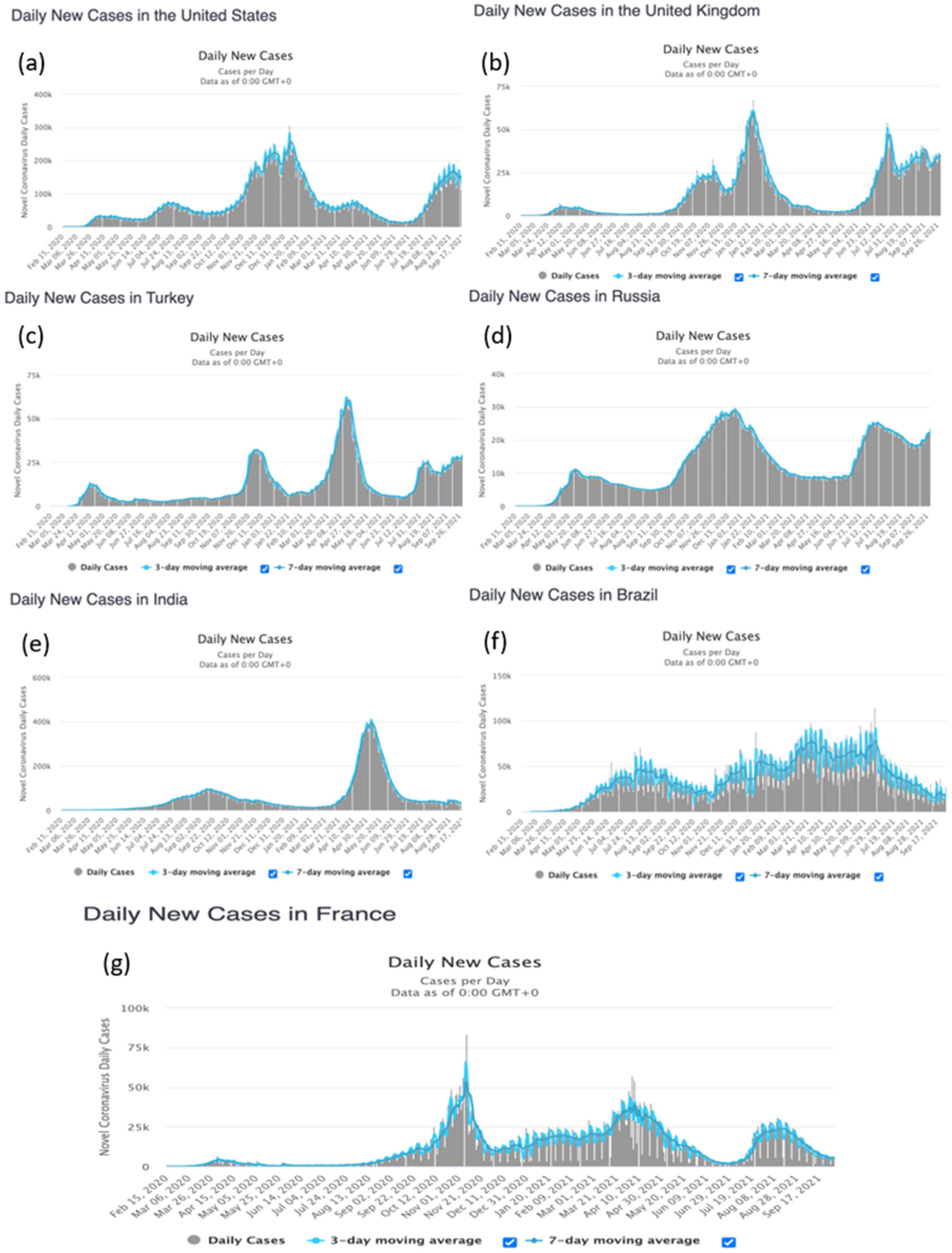
This article focuses on the application of deep learning and spectral analysis to epidemiology time series data, which has recently piqued the interest of some researchers. The COVID-19 virus is still mutating, particularly the delta and omicron variants, which are known for their high level of contagiousness, but policymakers and governments are resolute in combating the pandemic's spread through a recent massive vaccination campaign of their population. We used extreme machine learning (ELM), multilayer perceptron (MLP), long short-term neural network (LSTM), gated recurrent unit (GRU), convolution neural network (CNN) and deep neural network (DNN) methods on time series data from the start of the pandemic in France, Russia, Turkey, India, United states of America (USA), Brazil and United Kingdom (UK) until September 3, 2021 to predict the daily new cases and daily deaths at different waves of the pandemic in countries considered while using root mean square error (RMSE) and relative root mean square error (rRMSE) to measure the performance of these methods. We used the spectral analysis method to convert time (days) to frequency in order to analyze the peaks of frequency and periodicity of the time series data. We also forecasted the future pandemic evolution by using ELM, MLP, and spectral analysis. Moreover, MLP achieved best performance for both daily new cases and deaths based on the evaluation metrics used. Furthermore, we discovered that errors for daily deaths are much lower than those for daily new cases. While the performance of models varies, prediction and forecasting during the period of vaccination and recent cases confirm the pandemic's prevalence level in the countries under consideration. Finally, some of the peaks observed in the time series data correspond with the proven pattern of weekly peaks that is unique to the COVID-19 time series data.

| [1] | Seligmann H, Iggui S, Rachdi M, et al. (2020) Inverted covariate effects for mutated 2nd vs 1st wave Covid-19: high temperature spread biased for young. Medrxiv ppmedrxiv-20151878. |
| [2] | Demongeot J, Seligmann H (2020) SARS-CoV-2 and miRNA-like inhibition power. Med Hypotheses 144: 110245https://doi.org/10.1016/j.mehy.2020.110245. |
| [3] | Demongeot J, Griette Q, Magal P (2020) SI epidemic model applied to COVID-19 data in mainland China. Roy Soc Open Sci 7: 201878https://doi.org/10.1098/rsos.201878. |
| [4] | Soubeyrand S, Demongeot J, Roques L (2020) Towards unified and real-time analyses of outbreaks at country-level during pandemics. One Health 11: 100187https://doi.org/10.1016/j.onehlt.2020.100187. |
| [5] | Gaudart J, Landier J, Huiart L, et al. (2021) Factors associated with spatial heterogeneity of Covid-19 in France: a nationwide ecological study. The Lancet Public Health 6: e222-e231. https://doi.org/10.1016/S2468-2667(21)00006-2. |
| [6] | Oshinubi K, Al-Awadhi F, Rachdi M, et al. (2021) Data analysis and forecasting of COVID-19 pandemic in Kuwait based on daily observation and basic reproduction number dynamics. Kuwait J Sci Special Issue: 1-30. https://doi.org/10.48129/kjs.splcov.14501. |
| [7] | Oshinubi K, Ibrahim F, Rachdi M, et al. Functional data analysis: Transition from daily observation of COVID-19 prevalence in France to functional curves (2021) .https://doi.org/10.1101/2021.09.25.21264106. |
| [8] | Demongeot J, Oshinubi K, Rachdi M, et al. (2022) The application of ARIMA model to analyse incidence pattern in several countries. J Math Comput Sci 12: 10https://doi.org/10.28919/jmcs/6541. |
| [9] | Demongeot J, Oshinubi K, Seligmann H, et al. Estimation of daily reproduction rates in COVID-19 outbreak (2021) .https://doi.org/10.1101/2020.12.30.20249010. |
| [10] | Griette Q, Demongeot J, Magal P (2021) A robust phenomenological approach to investigate COVID-19 data for France. Math Appl Sci Eng 3: 149-218. https://doi.org/10.5206/mase/14031. |
| [11] | Worldometers (2021) .Available from: https://www.worldometers.info/coronavirus/. |
| [12] | Ahmed HM, Elbarkouky RA, Omar OAM, et al. (2021) Models for COVID-19 Daily confirmed cases in different countries. Mathematics 9: 659https://doi.org/10.3390/math9060659. |
| [13] | Tojanovic J, Boucher VG, Boyle J, et al. COVID-19 is not the flu: Four graphs from four countries (2021) .https://doi.org/10.3389/fpubh.2021.628479. |
| [14] | Bakhta A, Boiveau T, Maday Y, et al. (2021) Epidemiological forecasting with model reduction of compartmental models: application to the COVID-19 pandemic. Biology 10: 22https://doi.org/10.3390/biology10010022. |
| [15] | Abioye AI, Umoh MD, Peter OJ, et al. (2021) Forecasting of COVID-19 pandemic in Nigeria using real statistical data. Commun Math Biol Neurosci 2021: 2https://doi.org/10.28919/cmbn/5144. |
| [16] | Oshinubi K, Rachdi M, Demongeot J (2021) Analysis of daily reproduction rates of COVID-19 using current health expenditure as gross domestic product percentage (CHE/GDP) across countries. Healthcare 9: 1247https://doi.org/10.3390/healthcare9101247. |
| [17] | Deb S, Majumdar M (2020) A time series method to analyze incidence pattern and estimate reproduction number of COVID-19. ArXiv 2003.10655. |
| [18] | Hochreiter S, Schmidhuber J (1997) Long short-term memory. Neural Comput 9: 1735-1780. https://doi.org/10.1162/neco.1997.9.8.1735. |
| [19] | Chung J, Gulcehre C, Cho K, et al. (2014) Empirical evaluation of gated recurrent neural networks on sequence modeling. ArXiv 1412.3555. |
| [20] | Chimmula VKR, Zhang L (2020) Time series forecasting of COVID-19 transmission in Canada using LSTM networks. Chaos Soliton Fract 135: 109864https://doi.org/10.1016/j.chaos.2020.109864. |
| [21] | Yahia NB, Kandara MD, Saoud NBB Deep ensemble learning method to forecast COVID-19 outbreak (2020) .https://doi.org/10.21203/rs.3.rs-27216/v1. |
| [22] | Yang Z, Zeng Z, Wang K, et al. (2020) Modified SEIR and AI prediction of the epidemic trend of COVID-19 in China under public health interventions. J Thorac Dis 12: 165-174. http://dx.doi.org/10.21037/jtd.2020.02.64. |
| [23] | Cho K, Van Merriënboer B, Gulcehre C, et al. (2014) Learning phrase representations using RNN encoder-decoder for statistical machine translation. ArXiv 1406.1078. |
| [24] | Hochreiter S, Schmidhuber J (1996) LSTM can solve hard long time lag problems. Adv Neural Inf Proces Syst 9: 473-479. |
| [25] | Ren Y, Chen H, Han Y, et al. (2020) A hybrid integrated deep learning model for the prediction of citywide spatio-temporal flow volumes. Int J Geogr Inf Sci 34: 802-823. https://doi.org/10.1080/13658816.2019.1652303. |
| [26] | Zhang Y, Cheng T, Ren Y, et al. (2020) A novel residual graph convolution deep learning model for short-term network-based traffic forecasting. Int J Geogr Inf Sci 34: 969-995. https://doi.org/10.1080/13658816.2019.1697879. |
| [27] | Chollet F, Allaire JJ (2018) Deep Learning with R New York: Manning Publications. |
| [28] | Liu YH, Maldonado P (2018) R Deep Learning Projects: Master the Techniques to Design and Develop Neural Network Models in R UK: Packt Publishing. |
| [29] | Ma X, Dai Z, He Z, et al. (2017) Learning traffic as images: A deep convolutional neural network for large-scale transportation network speed prediction. Sensors 17: 818https://doi.org/10.3390/s17040818. |
| [30] | Jeong MH, Lee TY, Jeon S-B, et al. (2021) Highway speed prediction using gated recurrent unit neural networks. Appl Sci 11: 3059https://doi.org/10.3390/app11073059. |
| [31] | Omran NF, Abd-el Ghany SF, Saleh H, et al. (2021) Applying deep learning methods on time-series data for forecasting COVID-19 in Egypt, Kuwait and Saudi Arabia. Complexity 2021: 6686745https://doi.org/10.1155/2021/6686745. |
| [32] | Chae S, Kwon S, Lee D (2018) Predicting infectious disease using deep learning and big data. Int J Environ Res Public Health 15: 1596https://doi.org/10.3390/ijerph15081596. |
| [33] | Frank RJ, Davey N, Hunt SP (2001) Time series prediction and neural networks. J Intell Robot Syst 31: 91-103. https://doi.org/10.1023/A:1012074215150. |
| [34] | Gu J, Wang J, Kuen J, et al. (2017) Recent advances in convolutional neural networks. ArXiv 1512.07108. |
| [35] | Huang CJ, Chen Y-H, Ma Y, et al. Multiple-Input deep convolutional neural network model for COVID-19 forecasting in China (2020) .https://doi.org/10.1101/2020.03.23.20041608. |
| [36] | Miotto R, Wang R, Wang S, et al. (2018) Deep learning for healthcare: review, opportunities and challenges. Briengs Bioinformatics 19: 1236-1246. https://doi.org/10.1093/bib/bbx044. |
| [37] | Pascanu R, Gulcehre C, Cho K, et al. (2014) How to construct deep recurrent neural networks. ArXiv 1312.6026. |
| [38] | Ravi D, Wong D, Deligianni F, et al. (2017) Deep learning for health informatics. IEEE J Biomed Health 21: 4-21. https://doi.org/10.1109/JBHI.2016.2636665. |
| [39] | Priestley MB (1981) Spectral Analysis and Time Series, volume 1 of Probability and mathematical statistics: A series of monographs New York: Academic Press. |
| [40] | Priestley MB (1981) Spectral Analysis and Time Series, volume 2 of Probability and mathematical statistics: A series of monographs New York: Academic Press. |
| [41] | Parker RL, O'Brien MS (1997) Spectral analysis of vector magnetic field profiles. J Geophys Res 102: 24815-24824. https://doi.org/10.1029/97JB02130. |
| [42] | Percival D, Walden A (1993) Spectral Analysis for Physical Applications Cambridge: Cambridge University Press. |
| [43] | Prieto GA, Parker RL, Thomson DJ, et al. (2007) Reducing the bias of multitaper spectrum estimates. Geophys J Int 171: 1269-1281. https://doi.org/10.1111/j.1365-246X.2007.03592.x. |
| [44] | Thomson DJ (1982) Spectrum estimation and harmonic analysis. Proc IEEE 70: 1055-1096. https://doi.org/10.1109/PROC.1982.12433. |
| [45] | Rahim KJ, Burr WS, Thomson DJ (2014) Applications of Multitaper Spectral Analysis to Nonstationary Data [PhD thesis] Canada: Queen's University. |
| [46] | Ord K, Fildes R, Kourentzes N (2017) Principles of business forecasting New York: Wessex Press Publishing. |
| [47] | Kourentzes N, Barrow BK, Crone SF (2014) Neural network ensemble operators for time series forecasting. Expert Syst Appl 41: 4235-4244. https://doi.org/10.1016/j.eswa.2013.12.011. |
| [48] | Crone SF, Kourentzes N (2010) Feature selection for time series prediction – A combined filter and wrapper approach for neural networks. Neurocomputing 73: 1923-1936. https://doi.org/10.1016/j.neucom.2010.01.017. |
| [49] | Barrow D, Kourentzes N (2018) The impact of special days in call arrivals forecasting: A neural network approach to modelling special days. Eur J Oper Res 264: 967-977. https://doi.org/10.1016/j.ejor.2016.07.015. |
| [50] | Golyandina N, Korobeynikov A (2014) Basic singular spectrum analysis and forecasting with R. Comput Stat Data Anal 71: 934-954. https://doi.org/10.1016/j.csda.2013.04.009. |
| [51] | Zhang Z, Moore J (2011) New significance test methods for Fourier analysis of geophysical time series. Nonlin Processes Geophys 18: 643-652. https://doi.org/10.5194/npg-18-643-2011. |
| [52] | Shorten C, Khoshgoftaar TM, Furht B (2021) Deep Learning applications for COVID-19. J Big Data 8: 18https://doi.org/10.1186/s40537-020-00392-9. |
| [53] | Bergman A, Sella Y, Agre P, et al. (2020) Oscillations in U.S. COVID-19 incidence and mortality data reflect diagnostic and reporting factors. mSystems 5: e00544-20https://doi.org/10.1128/mSystems.00544-20. |
| [54] | Frescura FAM, Engelbrecht CA, Frank BS (2007) Significance tests for periodogram peaks. ArXiv 0706.2225. |
| [55] | Grzesica D, Wiecek P (2016) Advanced forecasting methods based on spectral analysis. Procedia Engineering 161: 253-258. https://doi.org/10.1016/j.proeng.2016.08.546. |
| [56] | Kalantari M (2021) Forecasting COVID-19 pandemic using optimal singular spectrum analysis. Chaos Soliton Fract 142: 110547https://doi.org/10.1016/j.chaos.2020.110547. |
| [57] | Castillo O, Melin PA (2021) Novel method for a COVID-19 classification of countries based on an intelligent fuzzy fractal approach. Healthcare 9: 196https://doi.org/10.3390/healthcare9020196. |
| [58] | Castillo O, Melin PA (2021) A new fuzzy fractal control approach of non-linear dynamic systems: The case of controlling the COVID-19 pandemics. Chaos Soliton Fract 151: 111250https://doi.org/10.1016/j.chaos.2021.111250. |
| [59] | Sun TZ, Wang Y (2020) Modeling COVID-19 epidemic in Heilongjiang province, China. Chaos Soliton Fract 138: 109949https://doi.org/10.1016/j.chaos.2020.109949. |
| [60] | Boccaletti S, Ditto W, Mindlin G, et al. (2020) Modeling and forecasting of epidemic spreading: the case of Covid-19 and beyond. Chaos Soliton Fract 135: 109794https://doi.org/10.1016/j.chaos.2020.109794. |
| [61] | Castillo O, Melin P (2020) Forecasting of COVID-19 time series for countries in the world based on a hybrid approach combining the fractal dimension and fuzzy logic. Chaos Soliton Fract 140: 110242https://doi.org/10.1016/j.chaos.2020.110242. |
| [62] | Mansour RF, Escorcia-Gutierrez J, Gamarra M, et al. (2021) Unsupervised deep learning based variation antoencoder model for COVID-19 diagnosis and classification. Pattern Recogn lett 151: 267-274. https://doi.org/10.1016/j.patrec.2021.08.018. |
| [63] | Jaiswal AK, Tiwari P, Kumar S, et al. (2019) Identifying pneumonia in chest X-rays: a deep learning approach. Measurement 145: 511-518. https://doi.org/10.1016/j.measurement.2019.05.076. |
| [64] | Wikipedia (2021) .Available from: https://www.google.com/search?q=neural+network+picture. |
| [65] | Ahmadian S, Jalali SMJ, Islam SMS, et al. (2021) A novel deep neuroevolution-based image classification method to diagnose coronavirus disease (COVID-19). Comput Biol Med 139: 104994https://doi.org/10.1016/j.compbiomed.2021.104994. |
| [66] | Jalali SMJ, Ahmadian M, Ahmadian S, et al. (2021) An oppositional-Cauchy based GSK evolutionary algorithm with a novel deep ensemble reinforcement learning strategy for COVID-19 diagnosis. Appl Soft Comput 111: 107675https://doi.org/10.1016/j.asoc.2021.107675. |
| [67] | Melin P, Monica JC, Sanchez D, et al. (2020) Multiple ensemble neural network models with fuzzy response aggregation for predicting COVID-19 time series: the case of Mexico. Healthcare 8: 181https://doi.org/10.3390/healthcare8020181. |
| [68] | Magal P, Seydi O, Webb G, et al. (2021) A model of vaccination for dengue in the Philippines 2016–2018. Front Appl Math Stat 7: 760259https://doi.org/10.3389/fams.2021.760259. |
| [69] | Oshinubi K, Rachdi M, Demongeot J Modelling of COVID-19 pandemic vis-à-vis some socio-economic factors (2021) .https://doi.org/10.1101/2021.09.30.21264356. |


Figures(11) / Tables(2)

Kayode Oshinubi, Augustina Amakor, Olumuyiwa James Peter, Mustapha Rachdi, Jacques Demongeot. Approach to COVID-19 time series data using deep learning and spectral analysis methods[J]. AIMS Bioengineering, 2022, 9(1): 1-21. doi: 10.3934/bioeng.2022001


 DownLoad: