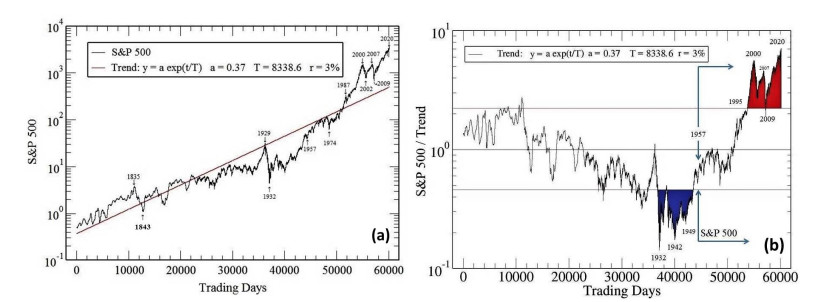
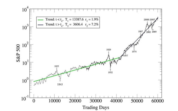
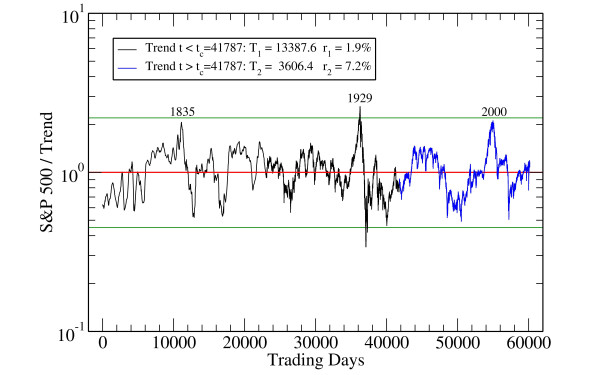
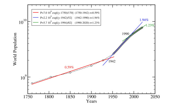
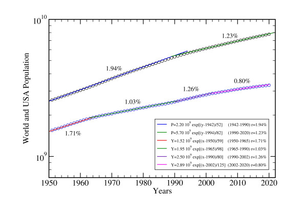
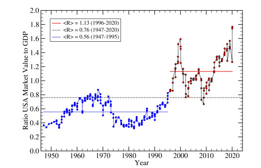
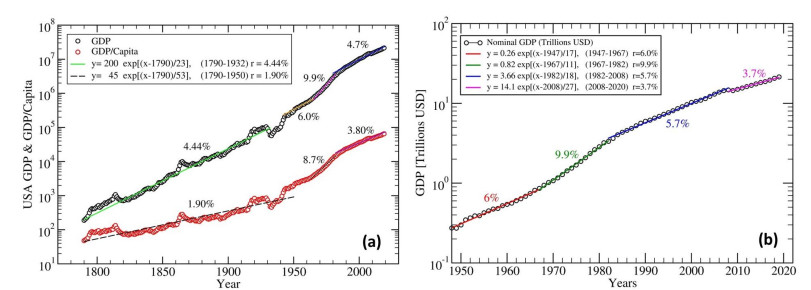
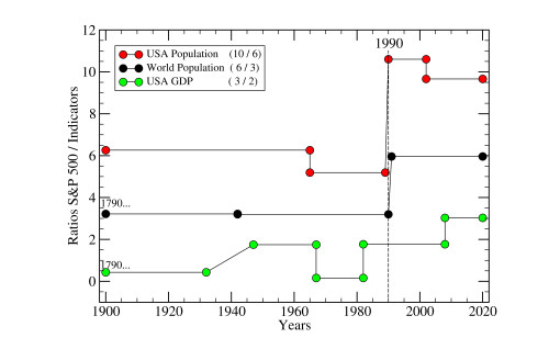
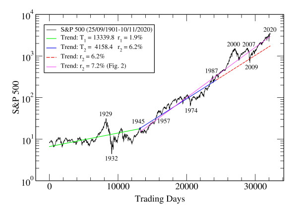
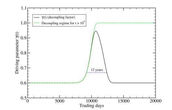
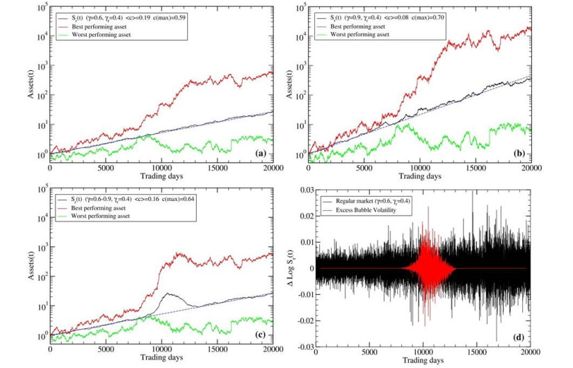
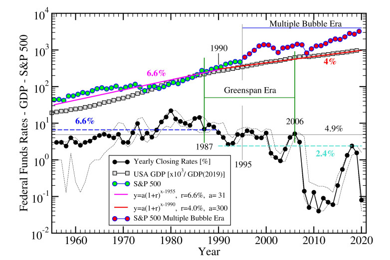
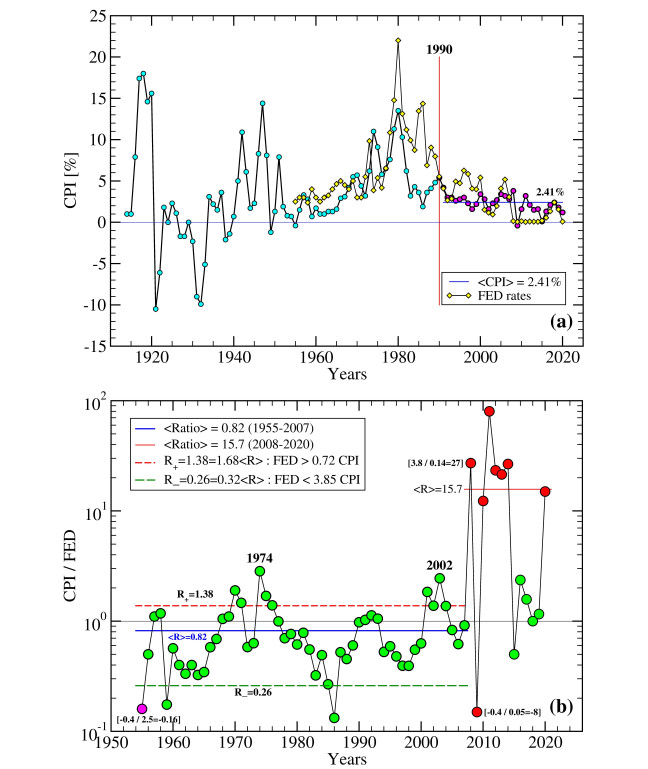
We discuss USA stock market data from 1789 until 2020, focusing our attention on the S&P 500 index (1957–2020). We find that the data can be split into two periods, (1789–1948) and (1948–2020), displaying roughly 2% and 7% growth rates, respectively. The index variations from each trend appear similar, suggesting some degree of stationarity in market fluctuations. We then correlate market behavior to macroeconomic data, such as world (and USA) population growth and gross domestic product (GDP), on different time horizons. The analysis signals that the S&P 500 might be overvalued, possibly undergoing a series of bubbles, since the 1990s. To understand this behavior, we introduce a model for bubbles, showing that they can be caused by a lack of correlations between stock prices and a virtual market index, the latter calculated self-consistently from the stock prices. We argue that variations, $ \Delta\gamma $, in the "bubble parameter" (or decoupling factor $ \gamma $), are anticorrelated to variations of the Federal Funds Rate (FFR), which may trigger a bubble phenomenon ($ \gamma\to1 $) when persistent rate cuts become too pronounced. The FFR are confronted with the consumer price index (CPI) in the period (1955–2020) as an attempt to complete the picture. Our analyses suggest that the strong departure of the S&P 500 from historical fundamental trends within (1990–2020) may reflect the development of financial anomalies, in part related to monetary policies, which should be carefully addressed in the near future.
Citation: Andrea Afify, Hector Eduardo Roman. Estimating market index valuation from macroeconomic trends[J]. Quantitative Finance and Economics, 2021, 5(2): 287-310. doi: 10.3934/QFE.2021013
We discuss USA stock market data from 1789 until 2020, focusing our attention on the S&P 500 index (1957–2020). We find that the data can be split into two periods, (1789–1948) and (1948–2020), displaying roughly 2% and 7% growth rates, respectively. The index variations from each trend appear similar, suggesting some degree of stationarity in market fluctuations. We then correlate market behavior to macroeconomic data, such as world (and USA) population growth and gross domestic product (GDP), on different time horizons. The analysis signals that the S&P 500 might be overvalued, possibly undergoing a series of bubbles, since the 1990s. To understand this behavior, we introduce a model for bubbles, showing that they can be caused by a lack of correlations between stock prices and a virtual market index, the latter calculated self-consistently from the stock prices. We argue that variations, $ \Delta\gamma $, in the "bubble parameter" (or decoupling factor $ \gamma $), are anticorrelated to variations of the Federal Funds Rate (FFR), which may trigger a bubble phenomenon ($ \gamma\to1 $) when persistent rate cuts become too pronounced. The FFR are confronted with the consumer price index (CPI) in the period (1955–2020) as an attempt to complete the picture. Our analyses suggest that the strong departure of the S&P 500 from historical fundamental trends within (1990–2020) may reflect the development of financial anomalies, in part related to monetary policies, which should be carefully addressed in the near future.

| [1] | Alexius A, Spång D (2018) Stock prices and GDP in the long run. J Appl Financ Bank 8: 107–126. |
| [2] |
Balcilar M, Gupta R, Wohar ME (2017) Common cycles and common trends in the stock and oil markets: Evidence from more than 150 years of data. Energy Econ 61: 72–86. doi: 10.1016/j.eneco.2016.11.003

|
| [3] |
Black F (1972) Capital market equilibrium with restricted borrowing. J Bus 45: 444–455. doi: 10.1086/295472
|
| [4] | Bogle JC (2017) The Little Book of Common Sense Investing: The Only Way to Guarantee Your Fair Share of Stock Market Returns, Prabhat Prakashan. |
| [5] |
Bonanno G, Caldarelli G, Lillo F, et al., (2003) Topology of correlation-based minimal spanning trees in real and model markets. Phys Rev E 68: 046130. doi: 10.1103/PhysRevE.68.046130
|
| [6] | Caspi I, Katzke N, Gupta R (2014) Date stamping historical oil price bubbles: 1876–2014. Stellenbosch Economic Working Papers: 20/14. |
| [7] |
Demirer R, Demos G, Gupta R, et al. (2019) On the predictability of stock market bubbles: evidence from LPPLS confidence multi-scale indicators. Quant Financ 19: 843–858. doi: 10.1080/14697688.2018.1524154
|
| [8] | Dose Ch, Porto M, Roman HE (2003) Autoregressive processes with anomalous scaling behavior: Applications to high-frequency variations of a stock market index. Phys Rev E 67: 063103. |
| [9] | Drożdż S, Grümmer F, Ruf F, et al. (2003) Log-periodic self-similarity: An emerging financial law? Phys A 324: 174–182. |
| [10] | Drożdż S, Kowalski R, Oświecimka P, et al. (2018) Dynamical variety of shapes in financial multifractality. Complexity (Hindawi) 2018: 1–13. |
| [11] |
Engle RF (1982) Autoregressive conditional heteroscedasticity with estimates of the variance of United Kingdom inflation. Econometrica 50: 987. doi: 10.2307/1912773
|
| [12] |
Flannery MJ, Protopapadakis AA (2002) Macroeconomic factors do influence aggregate stock returns. Rev Financ Stud 15: 751–782. doi: 10.1093/rfs/15.3.751
|
| [13] | Fortune P (1991) Stock market efficiency: an autopsy? New England Econ Rev 3/4: 17–40. |
| [14] |
Geanakoplos J, Magill M, Quinzii M (2004) Demography and the long-run predictability of the stock market. Brookings Pap Econ Act 2004: 241–325. doi: 10.1353/eca.2004.0010
|
| [15] | Graham B (1965) The Intelligent Investor, Prabhat Prakashan. |
| [16] |
Gündüz G (2021) Physical approach to elucidate stability and instability issues, and Elliott waves in financial systems: S&P-500 index as case study. Quant Financ Econ 5: 163–197. doi: 10.3934/QFE.2021008
|
| [17] | Kahneman D (2011) Thinking, Fast and Slow, Macmillan. |
| [18] | Lynch P, Rothchild J (2000) One Up On Wall Street: How To Use What You Already Know To Make Money In The Market, Simon and Schuster. |
| [19] | Malkiel BG (1999) A Random Walk Down Wall Street: Including a Life-cycle Guide To Personal Investing, WW Norton & Company. |
| [20] | Malkiel BG (2010) Bubbles in asset prices, The Oxford Handbook Of Capitalism, John Wiley & Sons. |
| [21] | Mandelbrot BB (1997) The variation of certain speculative prices, In: Fractals And Scaling In Finance, Springer, New York, NY, 371–418. |
| [22] | Markowitz HM (1959) Efficient Diversification of Investments–New York, John Wiley and Sons, New York. |
| [23] |
Phillips PCB, Yu J (2011) Dating the timeline of financial bubbles during the subprime crisis. Quant Econ 2: 455–491. doi: 10.3982/QE82
|
| [24] |
Roman HE, Porto M (2008) Fractional derivatives of random walks: Time series with long-time memory. Phys Rev E 78: 031127. doi: 10.1103/PhysRevE.78.031127
|
| [25] |
Roman HE, Porto M, Dose Ch (2008) Skewness, long-time memory, and non-stationarity: Application to leverage effect in financial time series. Europhys Lett 84: 28001. doi: 10.1209/0295-5075/84/28001
|
| [26] |
Roman HE, Albergante M, Colombo M, et al., (2006) Modeling cross correlations within a many-assets market. Phys Rev E 73: 036129. doi: 10.1103/PhysRevE.73.036129
|
| [27] | Sharpe WF (1964) Capital asset prices: A theory of market equilibrium under conditions of risk. J Financ 19: 425–442. |
| [28] |
Shiller RJ (2003) From efficient markets theory to behavioral finance. J Econ Perspect 17: 83–104. doi: 10.1257/089533003321164967
|
| [29] |
Sornette D, Cauwels P, Smilyanov G (2018) Can we use volatility to diagnose financial bubbles? Lessons from 40 historical bubbles. Quant Financ Econ 2: 486–594. doi: 10.3934/QFE.2018.1.486
|
| [30] | Wu TK (2012) Critical phenomena with renormalization group analysis of a hierarchical model of financial crashes. Master of Science Thesis, Simon Fraser University. |
| [31] |
Zhang Q, Sornette D, Balcilar M, et al. (2016) LPPLS bubble indicators over two centuries of the S&P 500 index. Phys A 458: 126–139. doi: 10.1016/j.physa.2016.03.103
|
Figures(14) / Tables(3)

Andrea Afify, Hector Eduardo Roman. Estimating market index valuation from macroeconomic trends[J]. Quantitative Finance and Economics, 2021, 5(2): 287-310. doi: 10.3934/QFE.2021013


 DownLoad: