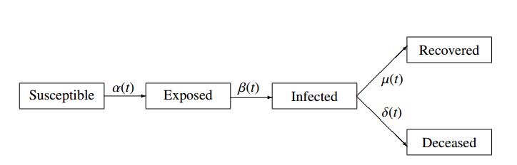
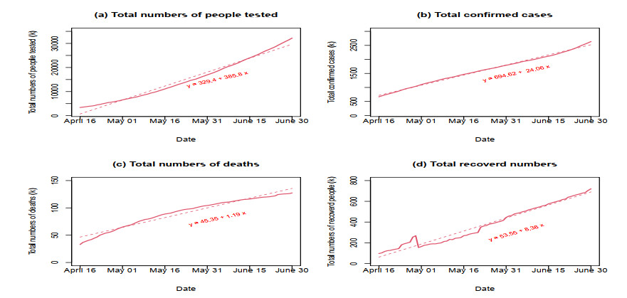
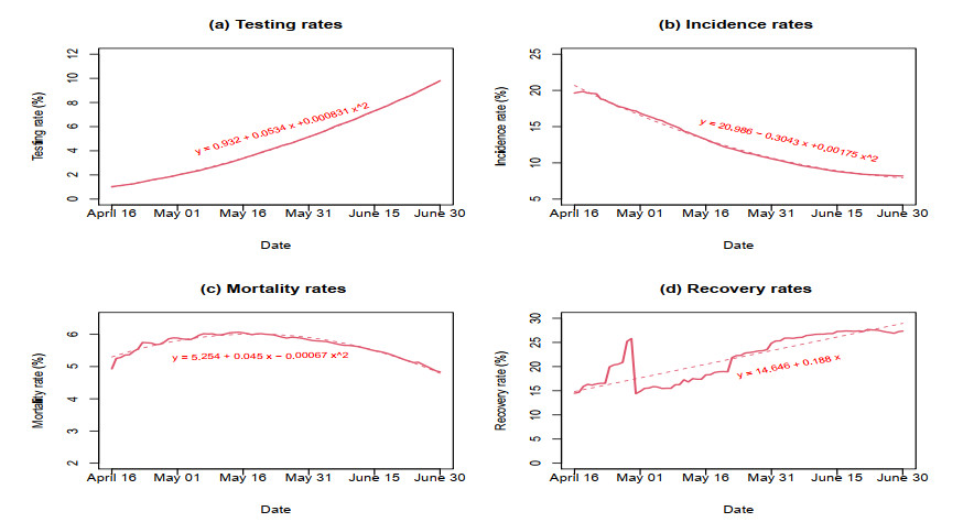
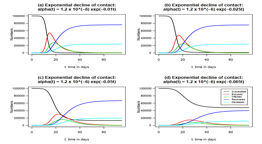
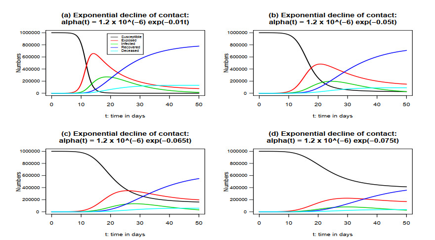
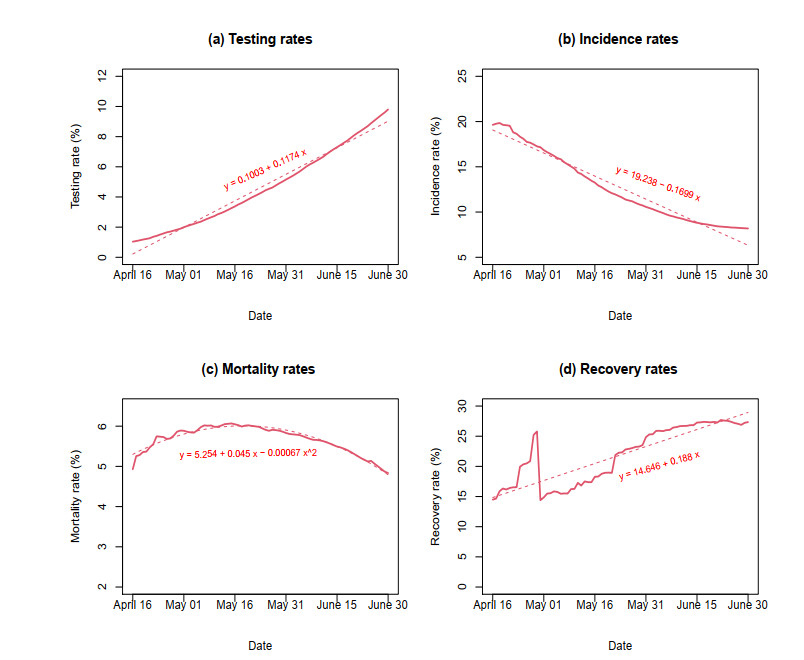
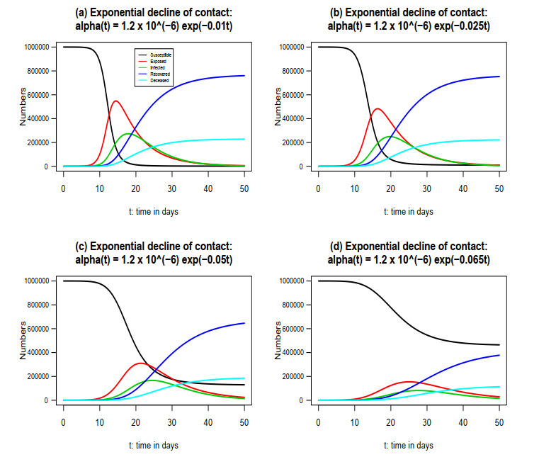
The emergence of coronavirus disease 2019 (COVID-19) demonstrates the importance of research on understanding and accurately modeling the transmission and spread of pandemic. In this paper, we consider a susceptible-exposed-infected-recovered-deceased (SEIRD) system of differential equations to describe relationship among the number of susceptible individuals, the number of exposed individuals who are transmitting the virus, the number of infected individuals among the exposed people, the number of recovered individuals from those infected, and the number of deaths from those infected in a town, state or country. Based on the empirical results of transmission process of COVID-19 in the United States from April 16th to June 30th, 2020, we consider a few cases of contact rate, incidence rate, recovery rate, and mortality rate to model the transmission and dynamics of the virus. Numerical analysis and analytical method are used to explore the dynamics and prediction of the pandemic.
Citation: Shuqi Wang, Wen Tang, Liyan Xiong, Mengyu Fang, Bingsong Zhang, Chi-Yang Chiu, Ruzong Fan. Mathematical modeling of transmission dynamics of COVID-19[J]. Big Data and Information Analytics, 2021, 6: 12-25. doi: 10.3934/bdia.2021002
The emergence of coronavirus disease 2019 (COVID-19) demonstrates the importance of research on understanding and accurately modeling the transmission and spread of pandemic. In this paper, we consider a susceptible-exposed-infected-recovered-deceased (SEIRD) system of differential equations to describe relationship among the number of susceptible individuals, the number of exposed individuals who are transmitting the virus, the number of infected individuals among the exposed people, the number of recovered individuals from those infected, and the number of deaths from those infected in a town, state or country. Based on the empirical results of transmission process of COVID-19 in the United States from April 16th to June 30th, 2020, we consider a few cases of contact rate, incidence rate, recovery rate, and mortality rate to model the transmission and dynamics of the virus. Numerical analysis and analytical method are used to explore the dynamics and prediction of the pandemic.

| [1] | World Health Organization (WHO), Coronavirus disease 2019 (COVID-19) situation reports. Available from: https://www.who.int/emergencies/diseases/novel-coronavirus-2019/situation-reports/. |
| [2] | Center for Disease Control and Prevention (CDC), Coronavirus disease 2019 (COVID-19). Available from: https://www.cdc.gov/coronavirus/2019-ncov/cases-updates/cases-in-us.html. |
| [3] | Center for Disease Control and Prevention (CDC), COVID-19 forecasts: cumulative deaths. Available from: https://www.cdc.gov/coronavirus/2019-ncov/covid-data/forecasting-us.html. |
| [4] |
Dong E, Du H and Gardner L, (2020) An interactive web-based dashboard to track COVID-19 in real time. Lancet Infect Dis 20: 533–543. doi: 10.1016/S1473-3099(20)30120-1

|
| [5] | USA daily state reports (csse_covid_19_daily_reports_us), the Johns Hopkins University. Available from: https://github.com/TWtangtang/COVID-19/tree/master/csse_covid_19_data. |
| [6] | The United States Census Bureau. Available from: https://www.census.gov/data/datasets/time-series/demo/popest/2010s-counties-total.html. |
| [7] |
Kissler SM, Tedijanto C, Goldstein E, et al. (2020) Projecting the transmission dynamics of SARS-CoV-2 through the postpandemic period. Science 368: 860–868. doi: 10.1126/science.abb5793
|
| [8] | Anderson RM, Anderson B and May RM, (1992) Infectious Diseases of Humans: Dynamics and Control, Oxford: Oxford University Press. |
| [9] |
Antia R, Regoes R, Koella JC, et al. (2003) The role of evolution in the emergence of infectious diseases. Nature 426: 658–661. doi: 10.1038/nature02104
|
| [10] | Bailey NTJ, (1975) The Mathematical Theory of Infectious Diseases and its Applications, London: Griffin. |
| [11] |
Bertozzi AL, Francob E, Mohlerd G, et al. (2020) The challenges of modeling and forecasting the spread of COVID-19. Proc Natl Acad Sci 117: 16732–16738. doi: 10.1073/pnas.2006520117
|
| [12] | Bjornstad ON, (2018) Epidemics: Models and Data using R, Springer. |
| [13] |
Brauer F, (2008) Compartmental models in epidemiology. Lect Notes Math Epidemiol 1945: 19–79. doi: 10.1007/978-3-540-78911-6_2
|
| [14] |
Chatterjee K, Chatterjee K, Kumar A, et al. (2020) Healthcare impact of COVID-19 epidemic in India: A stochastic mathematical model. Med J Armed Force 76: 147–155. doi: 10.1016/j.mjafi.2020.03.022
|
| [15] |
Earn DJD, (2008) A light introduction to modelling recurrent epidemics. Lect Notes Math Epidemiol 1945: 3–18. doi: 10.1007/978-3-540-78911-6_1
|
| [16] |
Earn DJD, Rohani P, Bolker BM, et al. (2000) A simple model for complex dynamical transitions in epidemics. Science 287: 667–670. doi: 10.1126/science.287.5453.667
|
| [17] |
Heesterbeek H, Anderson RM, Andreasen V, et al. (2015) Modeling infectious disease dynamics in the complex landscape of global health. Science 347: aaa4339. doi: 10.1126/science.aaa4339
|
| [18] |
Hethcote HW, (1976) Qualitative analyses of communicable disease models. Math Biosci 28: 335–356. doi: 10.1016/0025-5564(76)90132-2
|
| [19] |
Hethcote HW, (2000) The mathematics of infectious diseases. SIAM Rev 42: 599–653. doi: 10.1137/S0036144500371907
|
| [20] |
Hethcote HW and van den Driessche P, (1991) Some epidemiological models with nonlinear incidence. J Math Biol 29: 271–287. doi: 10.1007/BF00160539
|
| [21] |
Huppert A and Katriel G, (2013) Mathematical modelling and prediction in infectious disease epidemiology. Clin Microbiol Infect 19: 999–1005. doi: 10.1111/1469-0691.12308
|
| [22] |
Keeling MJ and Danon L, (2009) Mathematical modelling of infectious diseases. Br Med Bull 92: 33–42. doi: 10.1093/bmb/ldp038
|
| [23] | Keeling MJ and Rohani P, (2008) Modeling Infectious Diseases in Humans and Animals, Princeton University Press. |
| [24] | Kermack WO and McKendrick AG, (1927) A contribution to the mathematical theory of epidemics. Proc R Soc A 115: 700–721. |
| [25] | Li MY, Muldowney JS and van den Driessche P, (1991) Global stability of SEIRS models in epidemiology. Can Appl Math Quarterly 7: 409–425. |
| [26] |
Liu X and Stechlinski P, (2012) Infectious disease models with time-varying parameters and general nonlinear incidence rate. Appl Math Model 36: 1974–1994. doi: 10.1016/j.apm.2011.08.019
|
| [27] |
Miller JC, (2012) A note on the derivation of epidemic final sizes. Bull Math Biol 74: 2125–2141. doi: 10.1007/s11538-012-9749-6
|
| [28] | Miller JC, (2017) Mathematical models of SIR disease spread with combined non-sexual and sexual transmission routes. Infec Dis Model 2: 35–55. |
| [29] |
Osemwinyen AC and Diakhaby A, (2015) Mathematical modelling of the transmission dynamics of Ebola virus. Appl Comput Math 4: 313–320. doi: 10.11648/j.acm.20150404.19
|
| [30] | Rodrigues HS, (2016) Application of SIR epidemiological model: new trends. Int J Appl Math Inf 10: 92–97. |
| [31] |
Siettos CI and Russo L, (2013) Mathematical modeling of infectious disease dynamics. Virulence 4: 295–306. doi: 10.4161/viru.24041
|
| [32] |
Tang L, Zhou Y, Wang L, et al. (2020) A review of multi-compartment infectious disease models. Int Stat Rev 88: 462–513. doi: 10.1111/insr.12402
|
| [33] | Butcher JC, (2016) Numerical Methods for Ordinary Differential Equations, Chichester, United Kingdom: John Wiley & Sons. |
| [34] | Schittkowsky K, (2002) NNumerical Data Fitting in Dynamical Systems - A Practical Introduction with Applications and Software, Kluwer Academic Publishers. |
| [35] | Stoer J and Bulirsch R, (2013) Introduction to Numerical Analysis, New York, United States: Springer. |
| [36] | Allen LJS, (2003) An Introduction to Stochastic Processes with Applications to Biology, Prentice Hall. |
| [37] |
Allen LJS, (2008) An introduction to stochastic epidemic models. Lect Notes Math Epidemiol : 81–130. doi: 10.1007/978-3-540-78911-6_3
|
| [38] | Allen LJS, (2017) A primer on stochastic epidemic models: formulation, numerical simulation, and analysis. Infec Dis Model 2: 128–142. |
| [39] |
Aing RX, Liu JM, Cheung WKW, et al. (2016) Stochastic modelling of infectious diseases for heterogeneous populations. Infec Dis Poverty 5: 107. doi: 10.1186/s40249-016-0199-5
|
| [40] | Plank M, Binny RN, Hendy SC, et al. (2020) A stochastic model for COVID-19 spread and the effects of Alert Level 4 in Aotearoa New Zealand. medRxiv. |
| [41] |
AHadfield J, Colin Megill C, Bell1 SM, et al. (2018) Nextstrain: real-time tracking of pathogen evolution. Bioinformatics 34: 4121–4123. doi: 10.1093/bioinformatics/bty407
|
| [42] |
Quick J, Loman NJ, Duraffour S, et al. (2016) Real-time, portable genome sequencing for Ebola surveillance. Nature 530: 228–232. doi: 10.1038/nature16996
|
| [43] |
Sagulenko P, Puller V and Neher RA, (2018) Treetime: maximum-likelihood phylodynamic analysis. Virus Evol 4: vex042. doi: 10.1093/ve/vex042
|
| [44] |
Volz EM, Pond SLK, Ward MJ, et al. (2009) Phylodynamics of infectious disease epidemics. Genetics 183: 1421–1430. doi: 10.1534/genetics.109.106021
|
| [45] |
Volz EM, Koelle K and Bedford T, (2013) Viral phylodynamics. PLOS Comput Biol 9: e1002947. doi: 10.1371/journal.pcbi.1002947
|
Figures(7)

Shuqi Wang, Wen Tang, Liyan Xiong, Mengyu Fang, Bingsong Zhang, Chi-Yang Chiu, Ruzong Fan. Mathematical modeling of transmission dynamics of COVID-19[J]. Big Data and Information Analytics, 2021, 6: 12-25. doi: 10.3934/bdia.2021002


 DownLoad: