Processing math: 100%

Scalable Clustering by Truncated Fuzzy c-means

  • Most existing clustering algorithms are slow for dividing a large dataset into a large number of clusters. In this paper, we propose a truncated FCM algorithm to address this problem. The main idea behind our proposed algorithm is to keep only a small number of cluster centers during the iterative process of the FCM algorithm. Our numerical experiments on both synthetic and real datasets show that the proposed algorithm is much faster than the original FCM algorithm and the accuracy is comparable to that of the original FCM algorithm.

    Citation: Guojun Gan, Qiujun Lan, Shiyang Sima. Scalable Clustering by Truncated Fuzzy c-means[J]. Big Data and Information Analytics, 2016, 1(2): 247-259. doi: 10.3934/bdia.2016007

    Related Papers:

    [1] Jingya Wang, Ye Zhu . L2L control for memristive NNs with non-necessarily differentiable time-varying delay. Mathematical Biosciences and Engineering, 2023, 20(7): 13182-13199. doi: 10.3934/mbe.2023588
    [2] Kseniia Kravchuk, Alexander Vidybida . Non-Markovian spiking statistics of a neuron with delayed feedback in presence of refractoriness. Mathematical Biosciences and Engineering, 2014, 11(1): 81-104. doi: 10.3934/mbe.2014.11.81
    [3] Tianqi Yu, Lei Liu, Yan-Jun Liu . Observer-based adaptive fuzzy output feedback control for functional constraint systems with dead-zone input. Mathematical Biosciences and Engineering, 2023, 20(2): 2628-2650. doi: 10.3934/mbe.2023123
    [4] Gonzalo Robledo . Feedback stabilization for a chemostat with delayed output. Mathematical Biosciences and Engineering, 2009, 6(3): 629-647. doi: 10.3934/mbe.2009.6.629
    [5] Linni Li, Jin-E Zhang . Input-to-state stability of stochastic nonlinear system with delayed impulses. Mathematical Biosciences and Engineering, 2024, 21(2): 2233-2253. doi: 10.3934/mbe.2024098
    [6] Xiaoxiao Dong, Huan Qiao, Quanmin Zhu, Yufeng Yao . Event-triggered tracking control for switched nonlinear systems. Mathematical Biosciences and Engineering, 2023, 20(8): 14046-14060. doi: 10.3934/mbe.2023627
    [7] Tong Guo, Jing Han, Cancan Zhou, Jianping Zhou . Multi-leader-follower group consensus of stochastic time-delay multi-agent systems subject to Markov switching topology. Mathematical Biosciences and Engineering, 2022, 19(8): 7504-7520. doi: 10.3934/mbe.2022353
    [8] Dong Xu, Xinling Li, Weipeng Tai, Jianping Zhou . Event-triggered stabilization for networked control systems under random occurring deception attacks. Mathematical Biosciences and Engineering, 2023, 20(1): 859-878. doi: 10.3934/mbe.2023039
    [9] Yue Song, Yi Zhang, Song Yang, Na Li . Investigation on stability and controller design for singular bio-economic systems with stochastic fluctuations. Mathematical Biosciences and Engineering, 2021, 18(3): 2991-3005. doi: 10.3934/mbe.2021150
    [10] Xiaofeng Chen . Double-integrator consensus for a switching network without dwell time. Mathematical Biosciences and Engineering, 2023, 20(7): 11627-11643. doi: 10.3934/mbe.2023516
  • Most existing clustering algorithms are slow for dividing a large dataset into a large number of clusters. In this paper, we propose a truncated FCM algorithm to address this problem. The main idea behind our proposed algorithm is to keep only a small number of cluster centers during the iterative process of the FCM algorithm. Our numerical experiments on both synthetic and real datasets show that the proposed algorithm is much faster than the original FCM algorithm and the accuracy is comparable to that of the original FCM algorithm.


    In many industrial applications, due to the ubiquity of stochastic noise and nonlinear [1,2], real systems are often modelled by stochastic differential equations, which attracts researchers to pay more and more attention to the control of stochastic systems. Using the state-feedback, a closed-loop pole can be arbitrarily configured to improve the performance of the control systems. Therefore, some scholars research the problem of state-feedback stabilization for stochastic systems, e.g., reference [3] focuses on the cooperative control problem of multiple nonlinear systems perturbed by second-order moment processes in a directed topology. Reference [4] considers the case where the diffusion term and the drift term are unknown parameters for stochastic systems with strict feedback. Reference [5] studies stochastic higher-order systems with state constraints and [6] discusses output constrained stochastic systems with low-order and high-order nonlinear and stochastic inverse dynamics. However, it is often difficult to obtain all the state variables of the system directly, it is unsuitable for direct measurement or the measurement equipment is limited in economy and practicality, so the physical implementation of state-feedback is difficult. One of the solutions to this difficulty is to reconstruct the state of the system. At this time, scholars use an observer to investigate the output-feedback stabilization, e.g., reference [7] investigates the prescribed-time stability problem of stochastic nonlinear strict-feedback systems. Reference [8] focuses on stochastic strict feedback systems with sensor uncertainties. In addition, based on output-feedback, for nonlinear multiagent systems, a distributed output-feedback tracking controller is proposed in [9].

    It should be noted that all of the above results [7,8,9], Markovian switching is not considered in the design of output-feedback controller. However, as demonstrated by [10], switching system is a complex hybrid system, which consists of a series of subsystems and switching rules that coordinate the order of each subsystem. In real life, due to the aging of internal components, high temperature, sudden disturbance of external environment, operator error and other inevitable factors, the structure of many systems changes suddenly. Such systems can be reasonably modelled as differential equation with Markovian switching, see [11,12]. Recently, references [13] and [14] discuss the adaptive tracking problem and output tracking problem with Markovian switching respectively. Besides, as shown in [15], the power of the system changes because of factors such as the aging of the springs inside the boiler-turbine unit. Therefore, the research on the stability of stochastic nonlinear systems with time-varying powers has important practical significance. Reference [16] investigates the optimality and stability of high-order stochastic systems with time-varying powers. However, these results do not address the output-feedback stabilization for higher-order stochastic systems with both Markovian switching and time-varying powers.

    Based on these discussions, we aim to resolve the output-feedback stabilization for higher-order stochastic nonlinear systems with both Markovian switching and time-varying powers. The main contributions and characteristics of this paper are two-fold:

    1) The system model we take into account is more applicable than the existing results [7,8,9] and [12,13,14]. Different from the previous results [7,8,9], the stochastic system with Markovian switching is studied in this paper. Unlike previous studies in [12,13,14], we investigate the power is time-varying. The simultaneous existence of the Markov process and time-varying order makes the controller design process more complicated and difficult. More advanced stochastic analysis techniques are needed.

    2) We propose a new observer. The existence of Markovian switching and nondifferentiable time-varying power makes the observer constructed in [7,8,9] invalid. We use the time-varying power's bounds to construct a new observer, which can effectively observe the unmeasurable state and can deal with the nonlinear growth rate, while the existing observer can only deal with constant growth rate.

    The rest of this paper is listed as follows. The problem is formulated in Section 2. In Section 3, an output-feedback controller is designed. Section 4 is the stability analysis. A simulation is given in Section 5. The conclusions are collected in Section 6.

    Notations: R2 denotes the 2-dimensional space and the set of nonnegative real numbers is represented by R+. X denotes the matrix or vector, its transpose is represented by XT. |X| denotes the Euclidean norm of a vector X. When X is square, Tr{X} denotes its trace. The set of all functions with continuous ith partial derivatives is represented by Ci. Let C2,1(R2×R+×S;R+) represent all nonnegative functions V on R2×R+×S which are C2 in x and C1 in t.

    This paper studies the output-feedback stabilization for stochastic nonlinear systems with both Markovian switching and time-varying powers described by:

    dζ1=[ζ2]m(t)dt,dζ2=[u]m(t)dt+fTγ(t)(ˉζ2)dω,y=ζ1, (2.1)

    where ζ=ˉζ2=(ζ1,ζ2)TR2, yR and uR are the system state, control output and the input, respectively. The state ζ2 is unmeasurable. The function m(t):R+R+ is continuous and bounded, which satisfies 1m_m(t)ˉm with m_ and ˉm being constants. The powers sign function []α is defined as []α:=sign()||α with α(0,+). The functions fγ(t) is assumed to be smooth, and for all t0, the locally Lipschitz continuous in x uniformly. fγ(t)(t,0)=0. ω is an rdimensional standard Wiener process, which is defined on the complete probability space (Ω,F,Ft,P) with the filtration Ft satisfying the general conditions. γ(t) is a homogeneous Markov process on the probability space taking values in a space S={1,2,...,N}, which the generator Γ=(λij)N×N given by

    Pij(t)=P{γ(t+s)=i|γ(s)=j}={λijt+o(t)ifij,1+λijt+o(t)ifi=j, (2.2)

    where λij>0 is the transition rate from i to j if ij while λii=ΣNj=1,ijλij for any s,t0. Suppose the Markov process γ(t) is irrelevant to the ω(t).

    To implement the controller design, we need the following assumption.

    Assumption 2.1. There exists a non-negative smooth function ˜f(ζ1) such that

    |fγ(t)(ˉζ2)|(|ζ1|m(t)+12+|ζ2|m(t)+12)˜f(ζ1). (2.3)

    Remark 2.1. As we know, the existing results for stochastic systems with time-varying powers (e.g., [16]), neither the state-feedback control nor the output-feedback control, has considered Markovian switching. However, the structure of many physical systems in the actual system often mutates, which makes it necessary to study systems with both Markovain switching and time-varying powers. Therefore, compared with [16], the model we consider is more practical and more general.

    Remark 2.2. In Assumption 2.1, we can see that the power m(t) is time-varying and the growth rate ˜f(ζ1) is a nonlinear function. When m(t)=1 and ˜f(ζ1) is a constant, Assumption 2.1 is a linear growth condition. However, we consider that ˜f(ζ1) is a nonlinear function, which includes the constant case as a special case. The growth condition of Assumption 2.1 is broader than the linear growth condition. The time-varying power m(t) makes the design in [7,8,9] for time-invariant power invalid. In addition, the nonlinear growth rate ˜f(ζ1) makes the design in [7,8,9,17,18] for constant growth rate fail. A new design scheme should be proposed.

    In this section, we develop an output-feedback controller design for system (2.1). The process is divided into two steps:

    Firstly, we assume that all states are measurable and develop a state-feedback controller using backstepping technique.

    Secondly, we construct a reduced-order observer with a dynamic gain, and design an output-feedback controller.

    In this part, under Assumption 2.1, our objective is to develop a state-feedback controller design for the system (2.1).

    Step 1. Introducing the coordinate transformation ξ1=ζ1 and choosing V1=14ξ41, by using the infinitesimal generator defined in section 1.8 of [11], we have

    LV1ξ31[ζ2]m(t)+IIV1ξ31([ζ2]m(t)[ζ2]m(t))+ξ31[ζ2]m(t)+IIV1. (3.1)

    If we choose ζ2 as

    ζ2=c1/m_1ξ1:=α1ξ1, (3.2)

    we get

    ξ31[ζ2]m(t)=αm(t)1ξm(t)+31c1|ξ1|m(t)+3, (3.3)

    where α1=c1/m_11 is a constant with c11 being a design parameter.

    Substituting (3.3) into (3.1) yields

    LV1c1|ξ1|m(t)+3+ξ31([ζ2]m(t)[ζ2]m(t))+IIV1. (3.4)

    Step 2. Introducing the coordinate transformation ξ2=ζ2ζ2, and using Itô's differentiation rule, we get

    dξ2=([u]m(t)ζ2ζ1[ζ2]m(t))dt+fTγ(t)(ˉζ2)dω. (3.5)

    Choose V2=V1+14ξ42. From (3.4) and (3.5), we obtain

    LV2c1|ξ1|m(t)+3+ξ31([ζ2]m(t)[ζ2]m(t))+ξ32[u]m(t)ξ32ζ2ζ1[ζ2]m(t)+32ξ22|fTγ(t)(ˉζ2)|2+IIV2. (3.6)

    By (3.2) and using Lemma 1 in [19], we have

    ξ31([ζ2]m(t)[ζ2]m(t))ˉm(2ˉm2+2)(|ξ1|3|ξ2|m(t)+αˉm11|ξ1|m(t)+2|ξ2|). (3.7)

    By using Lemma 2.1 in [20], we get

    ˉm(2+2ˉm2)|ξ1|3|ξ2|m(t)16|ξ1|3+m(t)+β211|ξ2|3+m(t),ˉm(2+2ˉm2)αˉm11|ξ1|m(t)+2|ξ2|16|ξ1|3+m(t)+β212|ξ2|3+m(t), (3.8)

    where

    β211=ˉmm_+3(ˉm(2+2ˉm2))3+ˉmm_(3+m_18)3ˉm,β212=1m_+3(ˉm(2+2ˉm2)αˉm11)ˉm+3(m_+36(ˉm+2))(ˉm+2). (3.9)

    Substituting (3.8) into (3.7) yields

    ξ31([ζ2]m(t)[ζ2]m(t))13|ξ1|3+m(t)+β21|ξ2|3+m(t), (3.10)

    where β21=β211+β212 is a positive constant.

    By (3.2) and using Lemma 5 in [21], we get

    |ζ2|m(t)=|ξ2+ζ2|m(t)(|ξ2|+|α1ξ1|)m(t)2ˉm1(|ξ2|m(t)+|α1ξ1|m(t))2ˉm1αˉm1(|ξ2|m(t)+|ξ1|m(t)), (3.11)

    which means that

    |ζ1|m(t)+|ζ2|m(t)φ1(|ξ2|m(t)+|ξ1|m(t)), (3.12)

    where φ1=2ˉm1αˉm1+10 is a constant.

    By (3.11) and using Lemma 1 in [19], we have

    ξ32ζ2ζ1[ζ2]m(t)|ξ32||ζ2ζ1|2ˉm1αˉm1(|ξ2|m(t)+|ξ1|m(t))2ˉm1αˉm1|ζ2ζ1|(|ξ2|m(t)+3+|ξ32||ξ1|m(t)). (3.13)

    By using Lemma 2.1 in [20], we get

    2ˉm1αˉm1|ζ2ζ1||ξ32||ξ1|m(t)13|ξ1|3+m(t)+β221(ζ1)|ξ2|3+m(t), (3.14)

    where

    β221(ζ1)=3m_+3(2ˉm1αˉm1|ζ2ζ1|)ˉm+33(m_+33ˉm)ˉm3. (3.15)

    Substituting (3.14) into (3.13) yields

    ξ32ζ2ζ1[ζ2]m(t)13|ξ1|3+m(t)+β22(ζ1)|ξ2|3+m(t), (3.16)

    where β22(ζ1)=2ˉm1αˉm1|ζ2ζ1|+β221(ζ1) is a smooth function irrelevant to m(t).

    By (3.12), using Assumption 2.1 and Lemma 1 in [19], we get

    32ξ22|fTγ(t)(ˉζ2)|23˜f2(ζ1)|ξ2|2(|ζ1|m(t)+1+|ζ2|m(t)+1)3˜f2(ζ1)φ2(|ξ2|m(t)+3+|ξ2|2|ξ1|m(t)+1), (3.17)

    where φ2=2ˉmαˉm+11+10 is a constant.

    From Lemma 2.1 in [20], we obtain

    3˜f2(ζ1)φ2|ξ2|2|ξ1|m(t)+113|ξ1|m(t)+3+β231(ζ1)|ξ2|m(t)+3, (3.18)

    where

    β231(ζ1)=2m_+3(3˜f2(ζ1)φ2)ˉm+32(m_+33(ˉm+1))ˉm+12. (3.19)

    Substituting (3.18) into (3.17) yields

    32ξ22|fTγ(t)(ˉζ2)|213|ξ1|m(t)+3+β23(ζ1)|ξ2|m(t)+3, (3.20)

    where β23(ζ1)=3˜f2(ζ1)φ2+β231(ζ1)0 is a smooth function irrelevant to m(t).

    By using (3.6), (3.10), (3.16) and (3.20), we obtain

    LV2(c11)|ξ1|m(t)+3+ξ32([u]m(t)[x3]m(t))+ξ32[x3]m(t)+β2(ζ1)|ξ2|m(t)+3+IIV2, (3.21)

    where β2(ζ1)=β21(ζ1)+β22(ζ1)+β23(ζ1) is a smooth function irrelevant to m(t).

    Constructing the virtual controller as

    x3=(c2+β2(ζ1))1m_:=α2(ζ1)ξ2, (3.22)

    we have

    ξ32[x3]m(t)=αm(t)2(ζ1)ξm(t)+32(c2+β2(ζ1))ξm(t)+32, (3.23)

    where c2>0 is a constant and α2(ζ1)0 is a smooth function irrelevant to m(t).

    Substituting (3.23) into (3.21) yields

    LV2(c11)|ξ1|m(t)+3c2|ξ2|m(t)+3+ξ32([u]m(t)[x3]m(t))+IIV2. (3.24)

    In this part, we first design a reduced-order observer with a dynamic gain, then we design an output-feedback controller.

    Since ζ2 are unmeasurable, we construct the following observer

    dη=([u]m(t)L(ζ1)ζ1[η+L(ζ1)]m(t))dt, (3.25)

    where L(ζ1) is a smooth function, and L(ζ1)ζ1>0 is irrelevant to m(t).

    Defining e=ζ2L(ζ1)η and by the construction of the observer, we have

    de=L(ζ1)ζ1([η+L(ζ1)]m(t)[ζ2]m(t))dt+fTγ(t)(ˉζ2)dω. (3.26)

    Choose U=14e4. From (3.26), we get

    LU=e3L(ζ1)ζ1([η+L(ζ1)]m(t)[ζ2]m(t))+32e2|fTγ(t)(ˉζ2)|2+IIU. (3.27)

    By definition of e and lemma 2.2 in [22], we have

    e3L(ζ1)ζ1([η+L(ζ1)]m(t)[ζ2]m(t))12ˉm1L(ζ1)ζ1em(t)+3. (3.28)

    From (3.12), (3.17) and Assumption 2.1, we get

    32e2|fTγ(t)(ˉζ2)|23˜f2(ζ1)|e|2(|ζ1|m(t)+1+|ζ2|m(t)+1)3˜f2(ζ1)φ2(|e|2|ξ2|m(t)+1+|e|2|ξ1|m(t)+1). (3.29)

    By using Lemma 2.1 in [20], we have

    3˜f2(ζ1)φ2|e|2|ξ1|1+m(t)|ξ1|3+m(t)+β31(ζ1)|e|3+m(t),3˜f2(ζ1)φ2|e|2|ξ2|1+m(t)12|ξ2|3+m(t)+β32(ζ1)|e|3+m(t), (3.30)

    where

    β31(ζ1)=2m_+3(3˜f2(ζ1)φ2)ˉm+32(m_+3ˉm+1)ˉm+12,β32(ζ1)=2m_+3(3˜f2(ζ1)φ2)ˉm+32(3+m_2(1+ˉm))1+ˉm2. (3.31)

    Substituting (3.30) into (3.29) yields

    32e2|fTγ(t)(ˉζ2)|2|ξ1|m(t)+3+12|ξ2|m(t)+3+β3(ζ1)|e|m(t)+3, (3.32)

    where β3(ζ1)=β31(ζ1)+β32(ζ1)0 is a smooth function irrelevant to m(t).

    Substituting (3.28), (3.32) into (3.27) yields

    LU|ξ1|m(t)+3+12|ξ2|m(t)+3(12ˉm1L(ζ1)ζ1β3(ζ1))|e|m(t)+3+IIU. (3.33)

    Since ζ2 is unmeasurable, replace ζ2 in virtual controller x3 with η+L(ζ1), and we can get the controller as follows

    u=α2(ζ1)(η+L(ζ1)+α1ζ1). (3.34)

    By (3.22), (3.24) and (3.34), we obtain

    LV2(c11)|ξ1|m(t)+3c2|ξ2|m(t)+3+ξ32αˉm2(ζ1)([ξ2]m(t)[ξ2e]m(t))+IIV2. (3.35)

    By using Lemma 1 in [19], we have

    ξ32αˉm2(ζ1)([ξ2]m(t)[ξ2e]m(t))αˉm2(ζ1)ˉm(2ˉm2+2)(|ξ2|3|e|m(t)+|e||ξ2|m(t)+2). (3.36)

    By using Lemma 2.1 in [20], we get

    αˉm2(ζ1)ˉm(2ˉm2+2)|ξ2|3|e|m(t)14|ξ2|3+m(t)+β41(ζ1)|e|3+m(t),αˉm2(ζ1)ˉm(2ˉm2+2)|e||ξ2|2+m(t)14|ξ2|3+m(t)+β42(ζ1)|e|3+m(t), (3.37)

    where

    β41(ζ1)=ˉmm_+3(αˉm2(ζ1)ˉm(2ˉm2+2))ˉm+3m_(m_+312)3ˉm,β42(ζ1)=1m_+3(αˉm2(ζ1)ˉm(2ˉm2+2))ˉm+3(m_+34(ˉm+2))(ˉm+2). (3.38)

    Substituting (3.37) into (3.36) yields

    ξ32αˉm2(ζ1)([ξ2]m(t)[ξ2e]m(t))12|ξ2|3+m(t)+β4(ζ1)|e|3+m(t), (3.39)

    where β4(ζ1)=β41(ζ1)+β42(ζ1)0 is a smooth function irrelevant to m(t).

    By using (3.39) and (3.35), we have

    LV2(c11)|ξ1|m(t)+3(c212)|ξ2|m(t)+3+β4(ζ1)|e|m(t)+3+IIV2. (3.40)

    Choosing V(ξ1,ξ2,e)=V2(ξ1,ξ2)+U(e), by (3.33) and (3.40), we obtain

    LV(c12)|ξ1|m(t)+3(c21)|ξ2|m(t)+3(12ˉm1L(ζ1)ζ1β3(ζ1)β4(ζ1))|e|m(t)+3+IIV. (3.41)

    Let

    L(ζ1)=12ˉm1(c3ζ1+ζ10(β3(s)+β4(s))ds), (3.42)

    and the controller as

    u=α2(ζ1)(η+12ˉm1(c3ζ1+ζ10(β3(s)+β4(s))ds)+α1ζ1), (3.43)

    where c3>0 is a design parameter.

    By using (3.41) and (3.42), we can obtain

    LV(c12)|ξ1|m(t)+3(c21)|ξ2|m(t)+3c3|e|m(t)+3+IIV. (3.44)

    Remark 3.1. If m(t) is time-invariant and the growth rate is a constant rather than a smooth function, such as those in [7,8,9], from (3.32) and (3.39), β3 and β4 are constants irrelevant to ζ1. Then, the dynamic gain L(ζ) is a linear function of ζ1. We can design L(ζ1)=cζ1 by choosing the right parameter c to make LV in (3.41) negative definite. However, in this paper, the growth rate ˜f(ζ1) is a nonnegative smooth function and the m(t) is time-varying and non-differentiable, which makes the deducing of the dynamic gain much more difficult. To solve this problem, we introduce two constants m_ and ˉm, which are reasonably used in the design process, see (3.7) and (3.11). In this way, the dynamic gain (3.42) can be designed irrelevant to m(t), which is crucial to assure the effectiveness of the observer and controller. This is one of the main innovations of this paper.

    In this section, for the closed-loop system (2.1), (3.25) and (3.43), we first give a lemma, which is useful to prove the system has a unique solution. Then, we present the main results of the stability analysis.

    Lemma 4.1. For ζR, the function g(ζ)=[ζ]m(t) satisfies the locally Lipschitz condition.

    Proof. If ζ=0, we can get

    h+(0)=limζ0+h(ζ)h(0)ζ=0,h(0)=limζ0h(ζ)h(0)ζ=0. (4.1)

    Then, we have

    dhdζ|ζ=0=h+(0)=h(0)=0, (4.2)

    thus, h(ζ) is differentiable function in ζ=0 and so meets the locally Lipschitz condition in ζ=0.

    As ζ>0, we get

    h(ζ)=[ζ]m(t)=ζm(t). (4.3)

    For m(t)1, h(ζ) is differentiable function in ζ>0, so meets the locally Lipschitz condition in ζ>0. Similarly, as ζ<0, the conclusion is valid.

    Therefore, the conclusion holds for ζR.

    Next, we give the stability results.

    Theorem 4.1. Under Assumption 2.1, for the system (2.1), using the observer (3.25) and controller (3.43) with

    ci>3i,i=1,2,3, (4.4)

    we can get

    1) For each ζ(t0)=ζ0R2 and γ(t0)=i0S, the closed-loop system has an almost surely unique solution on [0,+);

    2) For any ζ0R2 and i0S, the closed-loop system is almost surely regulated to the equilibrium at the origin.

    Proof. By (2.1), (3.25), (3.43) and using Lemma 4.1, we can conclude that the closed-loop system satisfies the locally Lipschitz condition. By (3.2), (3.22), (3.25) and (3.42), we can get that ξ1,ξ2,η are bounded, which implies that ζ1 is bounded, which means that

    VR=inftt0,|ζ|>RV(ζ(t))R. (4.5)

    Through the verification of the controller development process, we choose appropriate design parameters ci to satisfy (4.4), and we can get IIV=0. For each l>0, the first exit time is defined as

    σl=inf{t:tt0,|ζ(t)|l}. (4.6)

    When tt0, choose tl=min{σl,t}. We can obtain that bounded |ζ(t)| on interval [t0,tl] a.s., which means that V(ζ) is bounded in the interval [t0,tl] a.s. By using (3.44), we can get that LV is bounded in the interval [t0,tl] a.s. By using Lemma 1.9 in [11], (3.44) and (4.4), we can obtain

    EV(ζ(tl))EV(ζ(t0)). (4.7)

    By (4.5), (4.7) and using Lemma 1 in [23], we can obtain conclusion (1).

    From (3.44), (4.5), by using Theorem 2.1 in [24], we can prove conclusion (2).

    In this section, a simulation example is given to show the availability of the control method.

    Study the stabilization for system with two modes. The Markov process γ(t) belongs to the space S={1,2} with generator Γ=(λij)2×2 given by λ11=2,λ12=2,λ21=1 and λ22=1. We have π1=13,π2=23. When γ(t)=1, the systems can be written as

    dζ1=[ζ2]32+12sintdt,dζ2=[u]32+12sintdt+ζ1sinζ2dω,y=ζ1, (5.1)

    where m(t)=32+12sint,m_=1,ˉm=2. When γ(t)=2, the systems are described by

    dζ1=[ζ2]2+sintdt,dζ2=[u]2+sintdt+12ζ21sinζ2dω,y=ζ1, (5.2)

    where m(t)=2+sint,m_=1,ˉm=3. Clearly, system (5.1) and (5.2) satisfy Assumption 2.1.

    According to the above design process, when γ(t)=1, the observer is constructed as

    dη=([u]32+12sintL(ζ1)ζ1[η+L(ζ1)]32+12sint)dt, (5.3)

    and the control is

    u=(c2+4ζ21)(η+L(ζ1)+c1ζ1), (5.4)

    where L(ζ1)=12(c3ζ1+6ζ21).

    When γ(t)=2, the observer is constructed as

    dη=([u]2+sintL(ζ1)ζ1[η+L(ζ1)]2+sint)dt, (5.5)

    and the control is

    u=(c2+4ζ1+12ζ21)(η+L(ζ1)+c1ζ1), (5.6)

    where L(ζ1)=14(c3ζ1+20ζ1+4ζ21).

    For simulation, we select c1=6,c2=6,c3=5, and the initial conditions as ζ1(0)=1,ζ2(0)=2,η(0)=5. We can obtain Figure 1, which illustrates that the signals of the closed-loop system (ζ1,ζ2,u,η,e) converge to zero. Specifically, the states and controller of the closed-loop system converge to zero. The observation error also converges to zero, which means that our constructed observer and controller are efficient. Figure 2 illustrates the jump of Markov process γ(t) in 1 and 2.

    Figure 1.  The responses of closed-loop systems (5.1)--(5.6).
    Figure 2.  The runs of the Markov process γ(t).

    Remark 5.1. It can be observed from the example that there are time-varying powers and Markovian switching in systems (5.1) and (5.2). For the output-feedback control of the system (5.1) and (5.2), the method in [7,8,9] fails since they can only deal with time-invariant powers without Markovian switching. To solve the difficulties caused by time-varying powers, we introduce constants 1, 2, and 1, 3 so that the design of the observer and controller is irrelevant to the power. This is one of the characteristics of our controller and observer design scheme (5.3)–(5.6).

    We investigate the output-feedback stabilization for stochastic nonlinear systems with both Markovian switching and time-varying powers in this paper. Compared with existing work, the system model considered in this paper is more general because it studies the time-varying power and Markovian switching, simultaneously. To achieve stabilization, we first design a state observer with a dynamic gain and an output-feedback controller, then use advanced stochastic analysis techniques to prove that the closed-loop system has an almost surely unique solution and the states are regulated to the origin almost surely. Even though there is no Markovian switching, the results in this paper are also new in the sense that we consider nonlinear growth rate, which is much more general than constant growth rate cases in [7,8,9].

    There are many related problems to be considered, such as how to extend the result to impulsive systems [25,26,27] and systems with arbitrary order.

    This work is funded by Shandong Province Higher Educational Excellent Youth Innovation team, China (No. 2019KJN017), and Shandong Provincial Natural Science Foundation for Distinguished Young Scholars, China (No. ZR2019JQ22).

    The authors declare there is no conflict of interest.

    [1] [ C. C. Aggarwal and C. K. Reddy (eds.), Data Clustering:Algorithms and Applications, CRC Press, Boca Raton, FL, USA, 2014.
    [2] [ D. Arthur and S. Vassilvitskii, k-means++:The advantages of careful seeding, in Proceedings of the Eighteenth Annual ACM-SIAM Symposium on Discrete Algorithms, SODA'07, Society for Industrial and Applied Mathematics, Philadelphia, PA, USA, 2007, 1027-1035.
    [3] [ J. C. Bezdek, R. Ehrlich and W. Full, FCM:The fuzzy c-means clustering algorithm, Computers & Geosciences, 10(1984), 191-203.
    [4] [ J. Bezdek, Pattern Recognition with Fuzzy Objective Function Algorithms, Kluwer Academic Publishers, Norwell, MA, USA, 1981.
    [5] [ A. Broder, L. Garcia-Pueyo, V. Josifovski, S. Vassilvitskii and S. Venkatesan, Scalable kmeans by ranked retrieval, in Proceedings of the 7th ACM International Conference on Web Search and Data Mining, WSDM'14, ACM, 2014, 233-242.
    [6] [ R. L. Cannon, J. V. Dave and J. Bezdek, Efficient implementation of the fuzzy c-means clustering algorithms, IEEE Transactions on Pattern Analysis and Machine Intelligence, PAMI-8(1986), 248-255.
    [7] [ T. W. Cheng, D. B. Goldgof and L. O. Hall, Fast fuzzy clustering, Fuzzy Sets and Systems, 93(1998), 49-56.
    [8] [ M. de Souto, I. Costa, D. de Araujo, T. Ludermir and A. Schliep, Clustering cancer gene expression data:A comparative study, BMC Bioinformatics, 9(2008), p497.
    [9] [ J. C. Dunn, A fuzzy relative of the ISODATA process and its use in detecting compact well-separated clusters, Journal of Cybernetics, 3(1973), 32-57.
    [10] [ G. Gan, Data Clustering in C++:An Object-Oriented Approach, Data Mining and Knowledge Discovery Series, Chapman & Hall/CRC Press, Boca Raton, FL, USA, 2011.
    [11] [ G. Gan, Application of data clustering and machine learning in variable annuity valuation, Insurance:Mathematics and Economics, 53(2013), 795-801.
    [12] [ G. Gan, A multi-asset Monte Carlo simulation model for the valuation of variable annuities, in Proceedings of the Winter Simulation Conference, 2015, 3162-3163.
    [13] [ G. Gan and S. Lin, Valuation of large variable annuity portfolios under nested simulation:A functional data approach, Insurance:Mathematics and Economics, 62(2015), 138-150.
    [14] [ G. Gan and M. K.-P. Ng, Subspace clustering using affinity propagation, Pattern Recognition, 48(2015), 1455-1464.
    [15] [ G. Gan and M. K.-P. Ng, Subspace clustering with automatic feature grouping, Pattern Recognition, 48(2015), 3703-3713.
    [16] [ G. Gan, Y. Zhang and D. K. Dey, Clustering by propagating probabilities between data points, Applied Soft Computing, 41(2016), 390-399.
    [17] [ R. J. Hathaway and J. C. Bezdek, Extending fuzzy and probabilistic clustering to very large data sets, Computational Statistics & Data Analysis, 51(2006), 215-234.
    [18] [ T. Havens, J. Bezdek, C. Leckie, L. Hall and M. Palaniswami, Fuzzy c-means algorithms for very large data, IEEE Transactions on Fuzzy Systems, 20(2012), 1130-1146.
    [19] [ M.-C. Hung and D.-L. Yang, An efficient fuzzy c-means clustering algorithm, in Proceedings IEEE International Conference on Data Mining, 2001, 225-232.
    [20] [ Z.-X. Ji, Q.-S. Sun and D.-S. Xia, A modified possibilistic fuzzy c-means clustering algorithm for bias field estimation and segmentation of brain MR image, Computerized Medical Imaging and Graphics, 35(2011), 383-397.
    [21] [ D. Jiang, C. Tang and A. Zhang, Cluster analysis for gene expression data:A survey, IEEE Transactions on Knowledge and Data Engineering, 16(2004), 1370-1386.
    [22] [ F. Klawonn, Fuzzy clustering:Insights and a new approach, Mathware & Soft Computing, 11(2004), 125-142.
    [23] [ J. F. Kolen and T. Hutcheson, Reducing the time complexity of the fuzzy c-means algorithm, IEEE Transactions on Fuzzy Systems, 10(2002), 263-267.
    [24] [ T. Kwok, K. Smith, S. Lozano and D. Taniar, Parallel fuzzy c-means clustering for large data sets, in Euro-Par 2002 Parallel Processing (eds. B. Monien and R. Feldmann), vol. 2400 of Lecture Notes in Computer Science, Springer, 2002, 365-374.
    [25] [ H. Liu, F. Zhao and L. Jiao, Fuzzy spectral clustering with robust spatial information for image segmentation, Applied Soft Computing, 12(2012), 3636-3647.
    [26] [ J. D. MacCuish and N. E. MacCuish, Clustering in Bioinformatics and Drug Discovery, CRC Press, Boca Raton, FL, 2010.
    [27] [ J. Macqueen, Some methods for classification and analysis of multivariate observations, in Proceedings of the 5th Berkeley Symposium on Mathematical Statistics andProbability (eds. L. LeCam and J. Neyman), University of California Press, Berkely, CA, USA, 1(1967), 281-297.
    [28] [ S. A. A. Shalom, M. Dash and M. Tue, Graphics hardware based efficient and scalable fuzzy cmeans clustering, in Proceedings of the 7th Australasian Data Mining Conference, 87(2008), 179-186.
    [29] [ A. Stetco, X.-J. Zeng and J. Keane, Fuzzy c-means++:Fuzzy c-means with effective seeding initalization, Expert Systems with Applications, 42(2015), 7541-7548.
  • This article has been cited by:

    1. Xinling Li, Xueli Qin, Zhiwei Wan, Weipeng Tai, Chaos synchronization of stochastic time-delay Lur'e systems: An asynchronous and adaptive event-triggered control approach, 2023, 31, 2688-1594, 5589, 10.3934/era.2023284
    2. Jingya Wang, Ye Zhu, L2L control for memristive NNs with non-necessarily differentiable time-varying delay, 2023, 20, 1551-0018, 13182, 10.3934/mbe.2023588
  • Reader Comments
  • © 2016 the Author(s), licensee AIMS Press. This is an open access article distributed under the terms of the Creative Commons Attribution License (http://creativecommons.org/licenses/by/4.0)
通讯作者: 陈斌, bchen63@163.com
  • 1. 

    沈阳化工大学材料科学与工程学院 沈阳 110142

  1. 本站搜索
  2. 百度学术搜索
  3. 万方数据库搜索
  4. CNKI搜索

Metrics

Article views(4459) PDF downloads(452) Cited by(4)

Figures and Tables

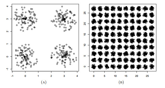
Figures(1)  /  Tables(5)

Other Articles By Authors

/

DownLoad:  Full-Size Img  PowerPoint
Return
Return

Catalog