Review Special Issues

Renewables exploitation for energy production and biomass use for electricity generation. A multi-parametric literature-based review

  • Nowadays, the provision of viable energy production and the energy autonomy are fundamental and utmost importance issues included in drawing the national strategic plan of both developing and developed countries. In parallel, the contentious role of fossil-based energy infrastructures, in the light of their high external costs of operation/use and the environmental depletion, have oriented current scientific research to find and exploit other energy sources that comply with increased pressure towards energy production, energy autonomy, and energy safety. Nevertheless, these preconditions of any energy mix introduced signify the importance of developing mature renewable energy technologies, which could enable sound and credible exploitation of any new-coming energy source, in the light of socio-economic acceptability and environmental sustainability. In parallel, the socio-economic traits, the know-how status, the technological maturity, the geo-morphologic conditions, and the well-being aspirations of each nation to its citizens consist also significant motives of energy-mix-schemes adaptation to a national level of analysis. According to the aforementioned statement, the present paper provides a four-fold overview upon: renewables’ exploitation for energy production in the global and European contexts, as well as biomass exploitation for electricity generation in a global-oriented and technology overview of the relevant literature. Conclusively, the main limitations and challenges that are derived from this four-fold literature overview, were also outlined.

    Citation: Grigorios L. Kyriakopoulos, Garyfallos Arabatzis, Miltiadis Chalikias. Renewables exploitation for energy production and biomass use for electricity generation. A multi-parametric literature-based review[J]. AIMS Energy, 2016, 4(5): 762-803. doi: 10.3934/energy.2016.5.762

    Related Papers:

    [1] David Moreno-Martos, Sean Foley, Benjamin Parcell, Dumitru Trucu, Raluca Eftimie . A computational investigation of COVID-19 transmission inside hospital wards and associated costs. Mathematical Biosciences and Engineering, 2022, 19(7): 6504-6522. doi: 10.3934/mbe.2022306
    [2] Qian Shen . Research of mortality risk prediction based on hospital admission data for COVID-19 patients. Mathematical Biosciences and Engineering, 2023, 20(3): 5333-5351. doi: 10.3934/mbe.2023247
    [3] Haonan Zhong, Wendi Wang . Mathematical analysis for COVID-19 resurgence in the contaminated environment. Mathematical Biosciences and Engineering, 2020, 17(6): 6909-6927. doi: 10.3934/mbe.2020357
    [4] Zhihao Zhang, Ting Zeng, Yijia Wang, Yinxia Su, Xianghua Tian, Guoxiang Ma, Zemin Luan, Fengjun Li . Prediction Model of hospitalization time of COVID-19 patients based on Gradient Boosted Regression Trees. Mathematical Biosciences and Engineering, 2023, 20(6): 10444-10458. doi: 10.3934/mbe.2023459
    [5] Sarita Bugalia, Vijay Pal Bajiya, Jai Prakash Tripathi, Ming-Tao Li, Gui-Quan Sun . Mathematical modeling of COVID-19 transmission: the roles of intervention strategies and lockdown. Mathematical Biosciences and Engineering, 2020, 17(5): 5961-5986. doi: 10.3934/mbe.2020318
    [6] Sarafa A. Iyaniwura, Musa Rabiu, Jummy F. David, Jude D. Kong . Assessing the impact of adherence to Non-pharmaceutical interventions and indirect transmission on the dynamics of COVID-19: a mathematical modelling study. Mathematical Biosciences and Engineering, 2021, 18(6): 8905-8932. doi: 10.3934/mbe.2021439
    [7] Xinmiao Rong, Liu Yang, Huidi Chu, Meng Fan . Effect of delay in diagnosis on transmission of COVID-19. Mathematical Biosciences and Engineering, 2020, 17(3): 2725-2740. doi: 10.3934/mbe.2020149
    [8] Jie Bai, Xiunan Wang, Jin Wang . An epidemic-economic model for COVID-19. Mathematical Biosciences and Engineering, 2022, 19(9): 9658-9696. doi: 10.3934/mbe.2022449
    [9] Yukun Tan, Durward Cator III, Martial Ndeffo-Mbah, Ulisses Braga-Neto . A stochastic metapopulation state-space approach to modeling and estimating COVID-19 spread. Mathematical Biosciences and Engineering, 2021, 18(6): 7685-7710. doi: 10.3934/mbe.2021381
    [10] Ziqiang Cheng, Jin Wang . Modeling epidemic flow with fluid dynamics. Mathematical Biosciences and Engineering, 2022, 19(8): 8334-8360. doi: 10.3934/mbe.2022388
  • Nowadays, the provision of viable energy production and the energy autonomy are fundamental and utmost importance issues included in drawing the national strategic plan of both developing and developed countries. In parallel, the contentious role of fossil-based energy infrastructures, in the light of their high external costs of operation/use and the environmental depletion, have oriented current scientific research to find and exploit other energy sources that comply with increased pressure towards energy production, energy autonomy, and energy safety. Nevertheless, these preconditions of any energy mix introduced signify the importance of developing mature renewable energy technologies, which could enable sound and credible exploitation of any new-coming energy source, in the light of socio-economic acceptability and environmental sustainability. In parallel, the socio-economic traits, the know-how status, the technological maturity, the geo-morphologic conditions, and the well-being aspirations of each nation to its citizens consist also significant motives of energy-mix-schemes adaptation to a national level of analysis. According to the aforementioned statement, the present paper provides a four-fold overview upon: renewables’ exploitation for energy production in the global and European contexts, as well as biomass exploitation for electricity generation in a global-oriented and technology overview of the relevant literature. Conclusively, the main limitations and challenges that are derived from this four-fold literature overview, were also outlined.


    There can be high mortality and morbidity for patients due to the spread of infections in hospitals (i.e., nosocomial or HAI) from infected patients to healthy patients, either directly through sharing the same rooms and environment, or indirectly through healthcare workers (HCWs) attending infected and susceptible patients. The novel coronavirus disease (COVID-19) that has been reported since January 2020, was shown to cause a relatively high prevalence of nosocomial infections: between 12.515% in the UK [1,2] and up to 44% in China [3]. In comparison, other coronaviruses such as SARS (Severe Acute Respiratory Syndrome, 2003) and MERS (Middle East Respiratory Syndrome, 2012), had estimated nosocomial infection prevalence of 36% and 56%, respectively [1].

    In UK hospitals, patients symptoms and results of real-time polymerase chain reaction (RT-PCR) inform targeted infection prevention and control (IPC) measures [1,2]. Patients who do not meet the clinical criteria for the COVID-19 disease may not be tested, and are usually admitted into shared bays, i.e., rooms of up to 6 beds that usually share the same bathroom facilities [2]. There can be problems with this approach, as highlighted in a recent study [2] in which it was shown that more than half of the patients who acquired COVID-19 in a hospital setting were identified as having been in the same hospital bay with other infected patients.

    There is also the issue of asymptomatic cases, which pose a particular risk for healthcare transmission. Various studies in the literature have estimated the proportion of asymptomatic COVID-19 infections: from 17.9% asymptomatic passengers on board of the Princess Cruises ship [4], to 30.8% asymptomatic Japanese nationals evacuated from Wuhan [5], 50–75% asymptomatic residents of an Italian village (Vo'Euganeo) [6], and even 81% asymptomatic passengers of an un-named cruise ship [7]. Since asymptomatic infections cannot be recognised if they are not confirmed by laboratory tests [5], it is highly likely that asymptomatic patients are found in hospitals, and they can be involved in the spread of COVID-19 inside these hospitals. In fact, a study in Beijing [8] showed that 5% of hospitalised patients were asymptomatic. This complicates the issue of nosocomial transmission of COVID-19, since hospitals do not test/re-test routinely all patients hospitalised for various interventions (not COVID-19 related).

    In regard to nosocomial transmissions, a 2015 report by the National Institute for Health Research [9] concluded that while hospital patients preferred a single-room accommodation, staff preferred a mix of single-rooms and shared-rooms accommodation. Moreover, a study examining hospital design [9] mentioned that it was impossible to perform an analysis of the impact of single-room hospital design on the transmission of HAIs, and given that some of the studies they cited showed a decrease in infections while other studies showed an increase in infections, the authors concluded that there was no clear evidence of the impact of single rooms on HAIs. Since some of the published COVID-19 studies [2] emphasised that 55% of HAIs were connected with infected patients in shared bays, it is important to understand COVID-19 transmission in these hospital bays.

    The common limitation of clinical studies that focus on the spread of COVID-19 inside hospitals (see, for example, [1,2,10]), is that they identify and count only PCR-symptomatic patients and not hospitalised patients that were exposed to the disease but were discharged before developing symptoms. Also, these studies cannot identify contacts between patients and staff, which might have had undiagnosed COVID-19 [2]. To address this lack of information, mathematical modelling and computational simulations are the perfect tool to test various scenarios regarding the mechanisms that can reduce the COVID-19 transmission in hospitals. Currently there are very few mathematical studies that focus on the nosocomial transmission of SARS-CoV-2 (despite the huge number of studies focused on the general viral spread through communities: e.g., from studies that focus only on symptomatic transmission [11,12,13,14,15], to studies that focus on both symptomatic and asymptomatic transmission [16,17,18,19], or transmission during the latent stages of the exposed period and during the symptomatic infectious period [14,20], transmission by various age classes [21,22], the impact of control measures such as school or workplace closures, or self-imposed and government-imposed social distancing measures [11,18,22,23,24,25]). We are aware of only one modelling study in [26], where the authors used a classical SEIR continuous model to investigate the transmission dynamics of COVID-19 in English hospitals, following interactions between patients and HCWs.

    Here we present a new study that considers a mathematical modelling approach to investigate the spread of COVID-19 among patients hospitalised in 4-bed versus 6-bed bays, which represents a standard bay structure in many hospitals in the UK; see also Figure 1. To this end we consider a network model that accounts for stochastic fluctuations between interconnected individuals inside the same hospital bay, where every single bed can be occupied by a susceptible, exposed, infectious or a recovered individual. With the help of this model we investigate computationally a variety of scenarios: from variations in the recovery and incubation periods; to the position of infected individuals in specific beds inside 6-bed bays; the effect of removing infected individuals from these bays; the effect of accommodating patients in single rooms; the effect of having asymptomatic individuals; and the role of periodic testing of hospitalised patients.

    Figure 1.  Typical distribution of beds in UK hospitals. Left: 6-bed bays; Right: 4-bed bays. In red it can be seen the distance between beds less than 2 m, while in green the distance between beds greater than 2 m.

    Since we are interested in investigating the transmission of infectious diseases (including COVID-19) across 4-bed and 6-bed hospital bays, which are the standard bays in many UK hospitals, in the following we consider an individual-based (network) model that tracks susceptible (S; i.e., patients vulnerable to develop an infection), exposed (E; i.e., patients incubating the virus), infected (I; i.e., patients that can transmit the disease) and recovered (R) individuals in each of the 4 or 6 beds inside these hospital bays. Following the approach in [27], each individual In,t is described by a set of characteristics, In,t=[Cn,1,t,Cn,2,t,...,Cn,m,t], where n=1,...N describes the number of individuals in the hospital bay, m is the number of characteristics, and t is the time. These characteristics are as follows:

    Cn,1,t is the epidemiological class. It can be 0 (susceptible), 1 (exposed), 2 (infected) or 3 (recovered).

    Cn,2,t is the bed at which the individual is placed.

    Cn,3,t is the time since the individual acquired the virus (start of the incubation period).

    Cn,4,t is the duration of the incubation period.

    Cn,5,t is the time since the individual has become infectious (virus transmission is now possible).

    Cn,6,t is the time that takes the individual to recover once becomes infectious.

    The following rules are used to update each of these states:

    Epidemiological class update:

    - A susceptible individual might become exposed with probability β if he/she interacts with an infected individual. Throughout this study we assume that the infection probability β depends on the distance between the susceptible individual and the infectious one. This modelling assumption is consistent with the clinical assumption of predominant transmission of SARS-CoV-2 via respiratory droplets [28]. Some recent studies have suggested that airborne transmission may be possible in certain circumstances, however to date the authors report that there is no perfect experimental data proving or disproving airborne transmission of SARS-CoV-2 [29]. Moreover, the evidence seems inconsistent with airborne transmission especially in well-ventilated spaces [29]. For this reason, and in accordance with current public health recommendations [30], in this study we assume that a distance of at least 2 m distance should be maintained to minimise the spread of SARS-CoV-2. Thus, here we consider the infection probability β to be a fixed number that depends on the distance between beds: probability is 1 if the distance is 0, probability is almost 0 if the distance is greater than 2; see the exponential distribution in Figure 2. The distance dij between two beds i and j (see also Figure 1) is given by matrices Dk=(dij), with i,j=1..k and k{4,6}:

    D4=(02.565.52.505.5665.502.55.562.50),D6=(01.536.35.75.51.501.55.75.55.731.505.55.76.36.35.75.501.535.75.55.71.501.55.55.76.331.50). (2.1)
    Figure 2.  Probability distribution of infection depending on the distance dij between beds i and j: β(dij)=exp(32dij). It is assumed here that the infectious disease spreads mainly though respiratory droplets, which fall to the ground rapidly within 1–2 m of the source person [29]. The case of airborne transmission, where aerosol particles persist in the air, can be modelled by a similar exponential function with a very low coefficient for dij – not investigated in this study, as explained in the main text.

    Therefore, the probability of becoming infected following the "contact" between individuals in beds i and j (where "contact" is understood in a very loose sense) is β(dij); see also Figure 2.

    We assume that there are a finite number of "contacts" within a day, and at each time step we simulate a "contact" between an infected individual and a susceptible one. Throughout this study we consider a time step Δt=0.1 days, which corresponds to an assumption of 10 contacts per day. (Note that changing the time step, i.e., the number of "contacts", impacts the speed at which the disease spreads but not the type of spread.)

    - An exposed individual becomes infected once his/her incubation period is finished (i.e., Cn,3,t>Cn,4,t).

    - An infected individual recovers if the time since he/she has been infected surpasses the expected duration of the infection (i.e., Cn,5,t>Cn,6,t).

    Incubation time update: If the individual is exposed, the incubation time update is increased by Δt at each iteration, until the individual becomes infectious.

    Incubation stage: We describe the duration of the incubation stage using an Erlang distribution with mean 1/σ and shape 2. Since the results obtained with this Erlang distribution are relatively similar to the results obtained with an exponential distribution (not shown here; for details see [31]), throughout this study we use only Erlang distributions.

    Infection time update: If the individual is infected, the infection time update is increased by Δt at each iteration, until the individual recovers.

    Recovery stage: Similar to the incubation stage, to describe the duration of the recovery stage we use an Erlang distribution with mean 1/γ and shape 2.

    Before we show the numerical results, we needs to discuss briefly the parameter values for which these results are obtained. Even if this model can be generally applied to the spread of various infectious diseases through hospital bays, here we focus on the spread of COVID-19. Therefore, the parameter values (i.e., mean recovery period, mean incubation period) are chosen for this particular disease, COVID-19, and are summarised in Table 1.

    Table 1.  Summary of model parameters used throughout this study. In the 4th column we show the most common values and ranges for the parameters that were found in the published literature (see references listed in the 5th column).
    Parameters (& units) Description Range Most common values References
    σ (day1) Incubation rate 0.0710.5 0.143, 0.192 [11,12,13,14,15,16,18,19,20,22,23,24,25,32,33,34,35,36,37,38]
    1/σ (day) Mean incubation period 214 7, 5.2 [11,12,13,14,15,16,18,19,20,22,23,24,25,32,33,34,35,36,37,38]
    γ (day1) Recovery rate 0.0550.621 0.1430.25 [11,12,13,14,15,16,18,19,21,22,23,24,32,33,35,36,37,39,40]
    1/γ (day) Mean recovery / infection period 1.6118 47 [11,12,13,14,15,16,18,19,21,22,23,24,32,33,35,36,37,39,40]

     | Show Table
    DownLoad: CSV

    For the numerical simulations presented here, we fix 1γ=7 days, 1σ=5.2 days, and we run the simulations up to Tmax=60 days. We run this network model 300 times, and we compute the mean and standard deviation of these 300 runs for individuals in each epidemiological state (i.e., susceptibles, exposed, infectives, recovered), for each of the 4-beds or 6-beds bays. We already mentioned before that the probability of infection β is given by a decaying exponential which depends on the distance between beds (see Figure 2). Finally, as initial conditions for these simulations, we assume that all patients are susceptible, with the exception of the individual placed in bed 2 (see Figure 1), who is exposed. This describes the situation where an individual, not being thought to have the disease (although they were exposed), is introduced into a hospital bay full of patients that can become infected. For simplicity, and to be able to compare the outcome of various simulations, we arbitrarily chose to place the exposed individual in bed 2. However, in Section 3.2 we discuss also what happens when we place the initial exposed individual in a different bed.

    We start this numerical investigation of our network model by assuming that hospitalised patients are accommodated in shared bays with either 4 beds or 6 beds. In Figure 3 we show the baseline dynamics of this model when an infected patient is hospitalised in bed 2 of a: (a), (b) 4-bed bay; (c), (d) 6-bed bay. We observe that in a 4-bed bay the average number of exposed and infected individuals decreases towards zero faster than in a 6-bed bay (see panels (a), (c)). Moreover, we note that for a 4-bed bay, individuals placed in beds 3 and 4 have an almost zero probability of becoming infected, when the original exposed patient was placed in bed 2 (see Figure 3(b)). For a 6-bed bay, individuals placed in beds 4, 5, and 6 have an almost zero probability of becoming infected, when the original exposed patient was placed in bed 2 (see Figure 3(d)). This means that the distance between the infected bed 2 and the beds on the opposite walls is large enough to avoid the infection.

    Figure 3.  Baseline dynamics for the network epidemiological model introduced in this study. (a) Average number of individuals per time, in a 4-bed bay; (b) Probability of being at each epidemiological state per bed, in a 4-bed bay; (c) Average number of individuals per time, in a 6-bed bay; (d) Probability of being at each epidemiological state per bed, in a 6-bed bay. Here we assume that 1/γ=7 days, 1/σ=5.2 days, Δt=0.1, and Tmax=60 days.

    In a 4-bed bay it does not matter where we place the first exposed individual, as the disease spreads equally in all beds due to the symmetry of bed distribution. However, in a 6-bed bay, it is important where we place the exposed individual: the disease is more likely to reach all the individuals in a room if the exposed individual is placed in beds 2 or 5. Next we compare how the disease evolves depending on where we place the first exposed individual in a 6-bed bay.

    In Figure 4 we assume that the first exposed individual is placed in bed 1, which is different from the case in Figure 3(b), (d) where we assumed that the first exposed individual was placed in bed 2.

    Figure 4.  The spread of infection in a 6-bed bay when the initial exposed individual is placed in bed 1. (a) Average number of individuals per time. (b) Probability of being at each epidemiological state per bed. We assume that 1/γ=7 days, 1/σ=5.2 days, Tmax=60 days, and Δt=0.1.

    We see that by placing the first exposed individual at bed 1, the disease spreads a bit slower compared to the case when this individual is placed in bed 2. More precisely, when we place him/her in bed 1, the average number of susceptible individuals decreases and reaches a steady value around t=35 days, whereas when we place him/her in bed 2 the steady value is reached around t=28 days.

    The parameters that characterise the transmission of COVID-19, e.g., mean incubation period and mean recovery period, are not fixed, with various studies showing different estimations; see Table 1. Here we focus on a 6-bed bay, and investigate the impact of incubation and recovery rates, showing only results for the minimum and the maximum values of these parameters. When varying the incubation rate we fix the mean recovery period to 1/γ=7 days, and when varying the recovery rate we fix the mean incubation period to 1/σ=5.2 days. (Here we do not vary β, since this parameter is given by the distance between beds; see caption of Figure 2.)

    Figure 5 shows model dynamics when we modify the recovery period. The most significant difference between the cases 1/γ=1.61 days and 1/γ=18 days is in the amplitude and shape of the infected curve. For the case where the recovery period is 18 days (Figure 5(c)) there is a time interval during which the number of infected individuals reaches a value of 2 (within one standard deviation). Since the recovery periods are larger (the mean recovery period is 18 days), there is more time in which susceptible individuals can become infected. This also affects the values of the average number of susceptible and recovered individuals. In terms of the probability of being at each epidemiological state per bed, there is a higher probability of becoming infected when the mean recovery period is 18 days (panels (d)), due to larger exposure to infected individuals.

    Figure 5.  Disease spread across a 6-bed bay, when we fix 1/σ=5.2 days and we vary 1/γ(1.61,18) days. (a) Average number of individuals per time when 1/γ=1.61 days; (b) Probability of being at each epidemiological state per bed, when 1/γ=1.61 days; (c) Average number of individuals per time when 1/γ=18 days; (d) Probability of being at each epidemiological state per bed, when 1/γ=18 days. As before we run simulations for Tmax=60 days, and Δt=0.1.

    The effects of varying the incubation period are shown in Figure 6. The most significant differences between the cases 1/σ=2 days and 1/σ=14 days can be found in the average numbers of exposed and infected individuals. When the mean incubation period is longer (Figure 6(c)), the mean value for the exposed and infected individuals reaches zero later in time. In terms of the probability of being at each epidemiological state per bed, the probability of being infected is higher for earlier times (t=10 days), when the mean incubation period is shorter (panels (c)).

    Figure 6.  Disease spread across a 6-bed bay, when we fix 1/γ=7 days and we vary 1/σ(2,14) days. (a) Average number of individuals per time when 1/σ=2 days; (b) Probability of being at each epidemiological state per bed, when 1/σ=2 days; (c) Average number of individuals per time when 1/σ=14 days; (d) Probability of being at each epidemiological state per bed, when 1/σ=14 days. As before we run simulations for Tmax=60 days, and Δt=0.1.

    Here we investigate the effect of removing from the bay every patient that is classified as infected (we remove this patient when the incubation period ends). We do this in order to reproduce the situation in which patients are transferred to separate COVID-19-only bays right at the moment they present clinical symptoms (assuming all of them are symptomatic individuals). Once we remove the infected patient, we place a new susceptible individual in the free bed. We emphasise that we modelled this out of mathematical interest (to keep the same number of patients in a bay and continue the simulations), as the standard clinical practice does not put a new person back in a bay with potential incubating patients.

    Since various studies reported pre-symptomatic transmission of SARS-CoV-2 during the incubation period [41,42,43], and following the approach in some published modelling studies [14,20] which accounted for the spread of infection during the latent period, in the following we assume that exposed individuals can transmit the disease, but at a much lower rate compared to the infected ones (we consider here an overlap between exposed and pre-symptomatic cases). Since we could not find in the literature any values for the probability of transmission, in this sub-section we set the probability of infection from the exposed individuals to be 20% of the probability of infection from the infected individuals. In Figure 7 we can see the differences between 4-bed bays and 6-bed bays.

    Figure 7.  Spread of the disease when infected individuals are removed from (a), (b) 4-bed bays; (c), (d) 6-bed bays. (a) Average number of individuals per time, in a 4-bed bay; (b) Probability of being at each epidemiological state, in a 4-bed bay. (c) Average number of individuals per time, in a 6-bed bay; (b) Probability of being at each epidemiological state, in a 6-bed bay. Here we assume that 1/γ=7 days, 1/σ=5.2 days, Tmax=60 days, and Δt=0.1.

    On one hand, in a 4-bed bay the disease disappears after a month. This is when we have 4 susceptible and 0 exposed in all the runs (Figure 7(a)) or the probability of being in the exposed state is zero for times greater than 30 days (Figure 7(b)). On the other hand, in a 6-bed bay the disease disappears after 50 days, which is when the probability of being in the exposed state is zero for t>50 days (Figure 7(d)). Both bays have in common the fact that the individuals across the aisle from the infected bed 2 (i.e., beds 3 and 4 in a 4-bed bay and beds 4, 5 and 6 in a 6-bed bay) do not become infected.

    Until now, we have assumed that patients in a hospital bay can become infected by interacting with exposed/infected individuals from the same bay. However, sometimes they have to share bathrooms with individuals from other bays, which increases the probability of becoming infected (it has been shown that the virus can survive for several hours on different surfaces [45]). Moreover, patients interact with hospital staff (doctors, nurses, etc.), who might transmit the disease with a very low probability [44], even if they follow the preventive measures (washing their hands, changing their clothes, wearing masks, etc.).

    To implement this aspect in our simulations, we note that the few studies that estimated the secondary attack rates for COVID-19 (defined as the probability that infection occurs among susceptibles, following contacts with an infectious person or infectious environment [46]) have shown wide ranges: from 0.45% in [47], to 35% in [48], and even 68.57% in [49]. The variability in the estimations for these attack rates might have been caused by the small sample sizes considered. To address this issue, a meta-analysis study focused on Taiwan patients [50] estimated a secondary attack rate for the nosocomial spread of SARS-CoV-2 between 0.73–2.93%. The authors of this study also emphasised the low attack rates that characterised the beginning of the epidemics (the data in [50] focused on cases between January and April 2020), and mentioned that higher attack rates were expected if the epidemics would continue. They also emphasised that in Taiwan the nosocomial attack rates were very low, due to staff training and increased awareness as a result of previous experiences with SARS.

    Based on these estimates, for our study we assume that each individual has a probability of 5% of becoming infected each day due to interactions with hospital staff and/or sharing the bathroom.

    In Figure 8 we see, for the first time in our simulations, that all patients have become infected in both 4-bed bays and 6-bed bays. Before considering interactions with staff members and sharing bathrooms, individuals at beds 3 and 4 (4-bed bay) and individuals at beds 4, 5 and 6 (6-bed bay) rarely became infected because the distance between beds was large enough to avoid the spread of the disease. However, if there are other ways of catching the disease, these patients will surely become infected. In fact, the probability of being recovered by t=60 days is 1 for all the beds in both bays.

    Figure 8.  Infection spread throughout (a), (b) 4-bed bays, and (c), (d) 6-bed bays, when we assume that each individual has a 5% probability of becoming infected due to interactions with staff members or sharing bathrooms. (a) Average number of individuals per time in a 4-bed bay; (b) Probability of being at each epidemiological state per bed, in a 4-bed bay. (c) Average number of individuals per time in a 6-bed bay; (d) Probability of being at each epidemiological state per bed, in a 6-bed bay. As before, we assume that 1/γ=7 days, 1/σ=5.2 days, Tmax=60 days, and Δt=0.1.

    In order to investigate the impact of disease spread following interactions with hospital staff, we now place only one individual in a single-bed room (which has an en-suite bathroom). Thus, the only way the patient can become infected is through interactions with the hospital staff. Since in this case we cannot talk about distance between beds, for the probability of infection β we assume that at the end of each day there is a fixed probability (5%) of becoming infected if the individual is susceptible.

    As stated in [51,52], the probability of infection is reduced by 85% when wearing masks. Here, we assume that the probability of infection is 5% per day when staff are wearing masks. Then we assume that the probability of becoming infected when staff are not wearing masks is 90%. In Figures 9(a) and (b) we show the probability of an individual (in a 1-bed room) of being at each epidemiological state when staff are wearing masks (sub-panel (a)) or not wearing masks (sub-panel (b)). It is clear that the use of masks increases the probability of the patient remaining in the susceptible state: from 0% after 10 days when the staff are not wearing masks, to 13% after 10 days when the staff are wearing masks.

    Figure 9.  Single-bed hospital rooms: probability of being at each epidemiological state. (a) When hospital staff are wearing masks, infections may occur each day with a probability of 5%. (b) When hospital staff are not wearing masks, infections may occur each day with a probability of 90%. As before, the duration of incubation and recovery periods follows an Erlang distribution with means 1/γ=7 days, 1/σ=5.2 days.

    Since it has been shown that a large number of the people infected with COVID-19 do not present with symptoms [6], but they can spread the virus efficiently [53] next we investigate the effects these asymptomatic individuals have on model dynamics. To this end, we split the infected individuals into "infected asymptomatic" and "infected symptomatic". Therefore, the epidemiological class Cn,1,t for each individuals can now take the following values: 0 (susceptible), 1 (exposed), 2 (infected asymptomatic), 3 (infected symptomatic) and 4 (recovered). Moreover, after the incubation period has passed, we randomly decide if the new individual is asymptomatic or symptomatic, with a maximum probability of 80% of being asymptomatic as suggested by various studies [7,54,6]. We assume that both exposed and infected asymptomatic individuals can transmit the disease, with the exposed individuals having a lower transmission probability (i.e., 20% lower, as considered also in Sub-section 3.4). We remove the infected symptomatic individuals the moment they become infected, and we remove the infected asymptomatic individuals after they test positive.

    Here, we compare the effects of running RT-PCR tests every day (Figure 10) or every 3 days (Figure 11) on hospitalised patients that have not been diagnosed with COVID-19. We see that it is better to run tests more often, as the probability of being susceptible (per bed) is higher when running tests every day (see panels (b), (d)). The results are similar for the 4-bay case and 6-bay case.

    Figure 10.  Disease spread when tests are run every day, and individuals have a 5% probability of becoming infected due to interaction with staff or by sharing bathrooms. (a) Average number of individuals per time, in a 4-bed bay. (b) Probability of being at each epidemiological state per bed, in a 4-bed bay. (c) Average number of individuals per time, in a 6-bed bay. (d) Probability of being at each epidemiological state per bed, in a 6-bed bay. As before, we assume that 1/γ=7 days, 1/σ=5.2 days, Tmax=60 days, Δt=0.1.
    Figure 11.  Disease spread when tests are run every 3 days, and individuals have a 5% probability of becoming infected due to interaction with staff or by sharing bathrooms. (a) Average number of individuals per time, in a 4-bed bay. (b) Probability of being at each epidemiological state per bed, in a 4-bed bay. (c) Average number of individuals per time, in a 6-bed bay. (d) Probability of being at each epidemiological state per bed, in a 6-bed bay. As before, we assume that 1/γ=7 days, 1/σ=5.2 days, Tmax=60 days, Δt=0.1.

    When running tests every 3 days (Figure 11), if we look at the infected asymptomatic individuals (in panels (a), (c)), sometimes we see two asymptomatic individuals in a bay. This is much higher compared to the case when tests are run every day, when the level of asymptomatics is zero (Figure 10(a), (c)). Moreover, for the case where tests are performed every 3 days, we note a periodic behaviour in the average number of individuals per time – caused by the removal of asymptomatics after they test positive.

    In this study we used modelling and computational approaches to investigate the question of the spread of an infectious disease through single rooms and shared hospital bays. This is an important aspect to be addressed due to the associated hospital costs of having single rooms or shared bays, and due to the very large numbers of patients that need to be hospitalised (with or without disease) in the context of a pandemic, as the one currently caused by SARS-CoV-2.

    To investigate the probability that an infectious disease would spread among patients hospitalised in single rooms and in shared hospital bays with 4 beds or 6 beds, we used a simple network model that considered the probability that each bed had a susceptible, exposed, infected (symptomatic or asymptomatic) or recovered individual. We built the model in steps, starting with the four epidemiological classes considered by the majority of early models for COVID-19 (i.e., susceptibles, exposed, infected and recovered; [14,17]). Then, we introduced asymptomatic infected individuals, to investigate their role in disease transmission across hospital bays (and how the results are different from the case where we assumed that all infected individuals are symptomatic – which was the standard assumption at the beginning of this pandemics). With the help of this model we tested a variety of scenarios: the effect of placing the initial exposed individual in different beds inside the 6-bed bay (see Figure 4); the effect of varying the recovery and incubation periods (see Figures 5 and 6); the effect of removing infected individuals from the bays (see Figure 7); the effect of interaction with members of staff and sharing bathrooms, thus increasing the daily probability of infection (see Figure 8); the role of asymptomatic individuals and the effect of frequent testing (every day or every 3 days) that can be used to identify asymptomatic individuals (see Figures 10 and 11); and finally the effect of having only 1 patient per room, in which case the probability of infection depends only on interactions with staff members (see Figure 9).

    We showed that patients hospitalised in single rooms have a higher probability to remain susceptible (i.e., not become infected) compared to patients in 4-bed bays; see Figures 9(a) and 8. We also showed that periodic testing combined with removing infected individuals from the bays reduces the probability of exposure and infection; see Figure 4.

    We conclude our theoretical study by emphasising that healthcare associated infectious diseases seem to spread slower in single (1-bed) rooms versus shared bays. Moreover, the COVID-19 infection spreads slower in 4-bed bays compared to 6-bed bays. This predictive result is important since a 2015 report by National Institute for Health Research on the impact of single-room accommodation on patient and staff experiences [9] concluded that there was no clear evidence of a reduction in HAIs through single rooms: while many studies showed a reduction in infection rates, other studies showed no differences or higher infection rates. In our theoretical study we have shown that, from an epidemiological point of view, there are differences in the disease transmission when there is a single patient per room, or multiple patients per room. Moreover, when there are multiple room occupancies, it is important to keep the number of patients as low as possible (e.g., 4 instead of 6), to slow down the spread of infectious diseases.

    Regarding periodic testing, current guidance [58] advocates for routine testing of asymptomatic HCWs every 7 days, depending on available testing capacity. Moreover, it is suggested that elective patients are to be tested for COVID-19 no more than 72 hours before admission, and cancer patients receiving long-course treatments should be tested every week [58]. The guidance from Health Protection Scotland [56] is that all patients over 70 years of age should tested for COVID-19 on admission to hospital. Moreover, the advice is that if the test results are negative, then the patients should be tested every 4 days until they are discharged [56]. Our simulation results investigated the effects of testing every 1–3 days. However, we emphasise that patient choice would need to be taken into account when developing policies for more frequent testing, as sampling has been reported to be uncomfortable. In addition, resources for testing would need to be increased in order for this to be feasible.

    Finally, since frequent RT-PCR testing may not be economically wise, laboratories certified under the Clinical Laboratory Improvement Amendments [57] may use a specimen pooling strategy, which allows laboratories to test more samples with fewer testing material and thus lower costs. This pooling strategy means combining respiratory samples from different people and conducting one laboratory test on the combined pool of samples [57].

    To conclude, in this study we have shown that transmission could be reduced by reducing the number of patients per room and by carrying out more regular testing. It is likely that a number of strategies will be required to reduce the risk of COVID-19 transmission and ensure the safe delivery of healthcare.

    It is a pleasure to acknowledge Wai-Lum Sung (graphic designer at the University of Aberdeen) for his assistance in the preparation of Figure 1, and Kathryn Brechin the Associate Nurse Director of Ninewells Hospital who created the first draft of Figure 1.

    The authors declare no conflict of interest.

    [1] Batel S, Devine-Wright P (2015) Towards a better understanding of people’s responses to renewable energy technologies: Insights from Social Representations Theory. Public Und Sci 24: 311-325.
    [2] Devine-Wright P (2010) Place attachment and the social acceptance of renewable energy technologies. Chapter 17 In: Psychological Approaches to Sustainability: Current Trends in Theory, Research and Applications. Edited by Victor Corral-Verdugo and Cirilo H. Garcia-Cadena. Nova Science Publishers Eds., 317-336.
    [3] Mallett A (2007) Social acceptance of renewable energy innovations: The role of technology cooperation in urban Mexico. Energ Policy 35: 2790-2798. doi: 10.1016/j.enpol.2006.12.008
    [4] Groba F, Cao J (2014) Chinese Renewable Energy Technology Exports: The Role of Policy, Innovation and Markets. Environ Resour Econ 60: 243-283.
    [5] Sung B, Song WY (2014) How government policies affect the export dynamics of renewable energy technologies: A subsectoral analysis. Energy 69: 843-859. doi: 10.1016/j.energy.2014.03.082
    [6] Zhang X, Chang S, Eric M (2012) Renewable energy in China: An integrated technology and policy perspective. Energ Policy 51: 1-6. doi: 10.1016/j.enpol.2012.09.071
    [7] Negro SO, Hekkert MP, Smits REHM (2008) Stimulating renewable energy technologies by innovation policy. Sci Public Policy 35: 403-416.
    [8] Jacobsson S, Lauber V (2006) The politics and policy of energy system transformation - Explaining the German diffusion of renewable energy technology. Energ Policy 34: 256-276.
    [9] Tsoutsos TD, Stamboulis YA (2005) The sustainable diffusion of renewable energy technologies as an example of an innovation-focused policy. Technovation 25: 753-761. doi: 10.1016/j.technovation.2003.12.003
    [10] Buckley JC, Schwarz PM (2003) Renewable energy from gasification of manure: An innovative technology in search of fertile policy. Environ Monit Assess 84: 111-127.
    [11] Hervás Soriano F, Mulatero F (2011) EU Research and Innovation (R&I) in renewable energies: The role of the Strategic Energy Technology Plan (SET-Plan). Energ Policy 39: 3582-3590.
    [12] Shen YC, Lin GTR, Li KP, et al. (2010) An assessment of exploiting renewable energy sources with concerns of policy and technology. Energ Policy 38: 4604-4616. doi: 10.1016/j.enpol.2010.04.016
    [13] Van Alphen K, Kunz HS, Hekkert MP (2008) Policy measures to promote the widespread utilization of renewable energy technologies for electricity generation in the Maldives. Renew Sust Energ Rev 12: 1959-1973. doi: 10.1016/j.rser.2007.04.009
    [14] Gan J, Smith CT (2006) A comparative analysis of woody biomass and coal for electricity generation under various CO­2 emission reductions and taxes. Biomass Bioenerg 30: 296-303.
    [15] Sung B, Song WY (2013) Causality between public policies and exports of renewable energy technologies. Energ Policy 55: 95-104. doi: 10.1016/j.enpol.2012.10.063
    [16] Garces E, Daim T (2013) An assessment of the impacts of government energy policy on energy technology, innovation, and security: The case of renewable technologies in the US electricity sector. Lect Notes Energ 16: 257-276.
    [17] Anderson D (1997) Renewable energy technology and policy for development. Annu Rev Energ Env 22: 187-215. doi: 10.1146/annurev.energy.22.1.187
    [18] Nisar A, Ruiz F, Palacios M (2013) Organisational learning, strategic rigidity and technology adoption: Implications for electric utilities and renewable energy firms. Renew Sust Energ Rev 22: 438-445.
    [19] García VG, Bartolomé MM (2010) Rural electrification systems based on renewable energy: The social dimensions of an innovative technology. Technol Soc 32: 303-311.
    [20] Tsai WT (2005) Current status and development policies on renewable energy technology research in Taiwan. Renew Sust Energ Rev 9: 237-253. doi: 10.1016/j.rser.2004.03.003
    [21] Abidin NZZ, Ibrahim JB (2015) Embracing renewables - Overcoming integration challenges from Malaysia's utility perspective. 2015 IEEE Eindhoven PowerTech, PowerTech, 2015: art. no. 7232373.
    [22] Loiter JM, Norberg-Bohm V (1999) Technology policy and renewable energy: Public roles in the development of new energy technologies. Energ Policy 27: 85-97.
    [23] Franco A, Salza P (2011) Perspectives for the long-term penetration of new renewables in complex energy systems: The Italian scenario. Environ Dev Sustainability 13: 309-330.
    [24] Amorim F, Martins MVM, Pereira Da Silva P (2010) A new perspective to account for renewables impacts in Portugal. 7th International Conference on the European Energy Market 2010, EEM 2010: art. no. 5558695.
    [25] Suwa A, Jupesta J (2012) Policy innovation for technology diffusion: A case-study of Japanese renewable energy public support programs. Sustainability Sci 7: 185-197. doi: 10.1007/s11625-012-0175-3
    [26] Vassilev SV, Vassileva CG, Vassilev VS (2015) Advantages and disadvantages of composition and properties of biomass in comparison with coal: An overview. Fuel 158: 330-350. doi: 10.1016/j.fuel.2015.05.050
    [27] Zandler H, Brenning A, Samimi C (2015) Potential of space-borne hyperspectral data for biomass quantification in an arid environment: Advantages and limitations. Remote Sens 7: 4565-4580.
    [28] Costa C, Rotsios K, Moshonas G, et al. (2014) Use of multivariate approaches in biomass energy plantation harvesting: Logistics advantages. Agr Eng Int: CIGR Journal May 2014: 71-80.
    [29] Bick S (2013) Skidding options for biomass operations: From big to small, each alternative has advantages and drawbacks. Northern Logger Timber Processor 62: 30-35.
    [30] Vassilev SV, Baxter D, Andersen LK, et al. (2013) An overview of the composition and application of biomass ash.: Part 2. Potential utilisation, technological and ecological advantages and challenges. Fuel 105: 19-39.
    [31] Talluri S, Subramanian MR, Christopher LP (2012) Advantages of thermophilic hydrogen production from lignocellulosic biomass. 2012 AIChE Annual Meeting Conference Proceedings: 1p.
    [32] Lanning CJ, Fridley JL (2012) Advances in woody biomass drying by taking advantage of surface properties. American Society of Agricultural and Biological Engineers Annual International Meeting 2012, ASABE 2012, 1: 715-723.
    [33] Santos CA, Ferreira ME, Lopes Da Silva T, et al. (2011) A symbiotic gas exchange between bioreactors enhances microalgal biomass and lipid productivities: Taking advantage of complementary nutritional modes. J Ind Microbiol Biotechn 38: 909-917. doi: 10.1007/s10295-010-0860-0
    [34] Hotchkiss R, Matts D, Riley G (2003) Co-combustion of Biomass with Coal - The Advantages and Disadvantages Compared to Purpose-built Biomass to Energy Plants. VGB PowerTech 83: 80-86.
    [35] Fransen B, De Kroon H (2001) Long-term disadvantages of selective root placement: Root proliferation and shoot biomass of two perennial grass species in a 2-year experiment. J Ecol 89: 711-722. doi: 10.1046/j.0022-0477.2001.00589.x
    [36] Nishiguchi S, Tabata T (2016) Assessment of social, economic, and environmental aspects of woody biomass energy utilization: Direct burning and wood pellets. Renew Sust Energ Rev 57: 1279-1286. doi: 10.1016/j.rser.2015.12.213
    [37] Miret C, Chazara P, Montastruc L, et al. (2016) Design of bioethanol green supply chain: Comparison between first and second generation biomass concerning economic, environmental and social criteria. Comput Chem Eng 85: 16-35. doi: 10.1016/j.compchemeng.2015.10.008
    [38] Singh J (2015) Overview of electric power potential of surplus agricultural biomass from economic, social, environmental and technical perspective - A case study of Punjab. Renew Sust Energ Rev 42: 286-297. doi: 10.1016/j.rser.2014.10.015
    [39] Cambero C, Sowlati T (2014) Assessment and optimization of forest biomass supply chains from economic, social and environmental perspectives - A review of literature. Renew Sust Energ Rev 36: 62-73. doi: 10.1016/j.rser.2014.04.041
    [40] Aylott MJ, Casella E, Farrall K, et al. (2010) Estimating the supply of biomass from short-rotation coppice in England, given social, economic and environmental constraints to land availability. Biofuels 1: 719-727. doi: 10.4155/bfs.10.30
    [41] Haughton AJ, Bond AJ, Lovett AA, et al. (2009) A novel, integrated approach to assessing social, economic and environmental implications of changing rural land-use: A case study of perennial biomass crops. J Appl Ecol 46: 315-322. doi: 10.1111/j.1365-2664.2009.01623.x
    [42] Fischer SL, Koshland CP, Young JA (2005) Social, economic, and environmental impacts assessment of a village-scale modern biomass energy project in Jilin province, China: local outcomes and lessons learned. Energ Sust Dev 9: 50-59. doi: 10.1016/S0973-0826(08)60499-8
    [43] Felker P (1984) Economic, environmental, and social advantages of intensively managed short rotation mesquite (Prosopis spp) biomass energy farms. Biomass 5: 65-77. doi: 10.1016/0144-4565(84)90070-2
    [44] Yilmaz Balaman T, Selim H (2015) A decision model for cost effective design of biomass based green energy supply chains. Bioresource Technol 191: 97-109. doi: 10.1016/j.biortech.2015.04.078
    [45] Dillibabu V, Natarajan E (2015) Green energy from biomass gasification. J Chem Pharm Sci 7: 182-185.
    [46] Hamzeh Y, Ashori A, Mirzaei B, et al. (2011) Current and potential capabilities of biomass for green energy in Iran. Renew Sust Energ Rev 15: 4934-4938. doi: 10.1016/j.rser.2011.07.060
    [47] Bhutto AW, Bazmi AA, Zahedi G (2011) Greener energy: Issues and challenges for Pakistan - Biomass energy prospective. Renew Sust Energ Rev 15: 3207-3219. doi: 10.1016/j.rser.2011.04.015
    [48] Demirbas T, Demirbas AH (2010) Bioenergy, green energy. biomass and biofuels. Energ Sources 32: 1067-1075.
    [49] Kaltschmitt M, Thrän D (2009) Biomass-based green energy generation. Chapter 7 In: Sustainable Solutions for Modern Economies. Edited by Martin Kaltschmitt and Daniela Thrän. Royal Society of Chemistry (RSC) Green Chemistry Eds., 86-124.
    [50] Jenner M (2008) Biomass energy outlook: How green is your carbon? BioCycle 49: 41.
    [51] Alfonsin V, Suarez A, Urrejola S, Miguez J, Sanchez A (2015) Integration of several renewable energies for internal combustion engine substitution in a commercial sailboat. Int J Hydrogen Energ 40: 6689-6701. doi: 10.1016/j.ijhydene.2015.02.113
    [52] Iniyan S, Suganthi L, Samuel AA (2006) Energy models for commercial energy prediction and substitution of renewable energy sources. Energ Policy 34: 2640-2653. doi: 10.1016/j.enpol.2004.11.017
    [53] Lombard A, Ferreira SLA (2015) The spatial distribution of renewable energy infrastructure in three particular provinces of South Africa. Bull Geogr 30: 71-85.
    [54] Palmas C, Siewert A, von Haaren C (2015) Exploring the decision-space for renewable energy generation to enhance spatial efficiency. Environ Impact Assess Rev 52: 9-17. doi: 10.1016/j.eiar.2014.06.005
    [55] Young M (2015) Building the blue economy: The role of marine spatial planning in facilitating offshore renewable energy development. Int J Marine Coastal Law 30: 148-173. doi: 10.1163/15718085-12341339
    [56] Güngör-Demirci G (2015) Spatial analysis of renewable energy potential and use in Turkey. J Renew Sust Energ 2015, 7: art. no. 013126.
    [57] Campbell MS, Stehfest KM, Votier SC, Hall-Spencer JM (2014) Mapping fisheries for marine spatial planning: Gear-specific vessel monitoring system (VMS), marine conservation and offshore renewable energy. Marine Policy 45: 293-300. doi: 10.1016/j.marpol.2013.09.015
    [58] Karakostas S, Economou D (2014) Enhanced multi-objective optimization algorithm for renewable energy sources: Optimal spatial development of wind farms. Int J Geogr Inform Sci 28: 83-103. doi: 10.1080/13658816.2013.820829
    [59] Wang Q, M’Ikiugu MM, Kinoshita I (2014) A GIS-based approach in support of spatial planning for renewable energy: A case study of Fukushima, Japan. Sustainability 6: 2087-2117. doi: 10.3390/su6042087
    [60] Behringer S, Upmann T (2014) Optimal harvesting of a spatial renewable resource. J Econ Dyn Control 42: 105-120. doi: 10.1016/j.jedc.2014.03.008
    [61] Davies IM, Watret R, Gubbins M (2014) Spatial planning for sustainable marine renewable energy developments in Scotland. Ocean Coastal Manage 99: 72-81. doi: 10.1016/j.ocecoaman.2014.05.013
    [62] Yang C, Ogden JM (2013) Renewable and low carbon hydrogen for California-Modeling the long term evolution of fuel infrastructure using a quasi-spatial TIMES model. Int J Hydrogen Energ 38: 4250-4265. doi: 10.1016/j.ijhydene.2013.01.195
    [63] Baltas AE, Dervos AN (2012) Special framework for the spatial planning & the sustainable development of renewable energy sources. Renew Energ 48: 358-363.
    [64] Haller M, Ludig S, Bauer N (2012) Decarbonization scenarios for the EU and MENA power system: Considering spatial distribution and short term dynamics of renewable generation. Energ Policy 47: 282-290. doi: 10.1016/j.enpol.2012.04.069
    [65] Katsaprakakis DA, Christakis DG (2016) The exploitation of electricity production projects from Renewable Energy Sources for the social and economic development of remote communities. the case of Greece: An example to avoid. Renew Sust Energ Rev 54:341-349.
    [66] Kyriakopoulos GL, Arabatzis G (2016) Electrical energy storage systems in electricity generation: Energy policies, innovative technologies, and regulatory regimes. Renew Sust Energ Rev 56:1044-1067.
    [67] Zografidou E, Petridis K, Arabatzis G, et al. (2016) Optimal design of the renewable energy map of Greece using weighted goal-programming and data envelopment analysis. Comput Oper Res 66: 313-326. doi: 10.1016/j.cor.2015.03.012
    [68] Ntona E, Arabatzis G, Kyriakopoulos GL (2015) Energy saving: Views and attitudes of students in secondary education. Renew Sust Energ Rev 46: 1-15. doi: 10.1016/j.rser.2015.02.033
    [69] Arabatzis G, Petridis K, Galatsidas S, et al. (2013) A demand scenario based fuelwood supply chain: A conceptual model. Renew Sust Energ Rev 25: 687-697. doi: 10.1016/j.rser.2013.05.030
    [70] Arabatzis G, Malesios Ch (2013) Pro-Environmental attitudes of users and not users of fuelwood in a rural area of Greece. Renew Sust Energ Rev 22: 621-630. doi: 10.1016/j.rser.2013.02.026
    [71] Balaras CA, Dascalaki EG, Droutsa P, et al. (2013) Hellenic renewable energy policies and energy performance of residential buildings using solar collectors for domestic hot water production in Greece. J Renew Sust Energ 5: art. no. 041813.
    [72] Kyriakopoulos G, Chalikias M (2013) The Investigation of Woodfuels’ Involvement in Green Energy Supply Schemes at Northern Greece: The Model Case of the Thrace Prefecture. Procedia Technol 8: 445-452.
    [73] Menegaki AN, Gurluk S (2013) Greece & Turkey; assessment and comparison of their renewable energy performance. Int J Energ Econ Policy 3: 367-383.
    [74] Metaxas A, Tsinisizelis M (2013) The development of renewable energy governance in Greece. Examples of a failed (?) policy. Lecture Notes Energy 23: 155-168.
    [75] Mondol JD, Koumpetsos N (2013) Overview of challenges, prospects, environmental impacts and policies for renewable energy and sustainable development in Greece. Renew Sust Energ Rev 23: 431-442. doi: 10.1016/j.rser.2013.01.041
    [76] Zafirakis D, Chalvatzis K, Kaldellis JK (2013) Socially just support mechanisms for the promotion of renewable energy sources in Greece. Renew Sust Energ Rev 21: 478-493. doi: 10.1016/j.rser.2012.12.030
    [77] Arabatzis G, Kitikidou K, Tampakis S, et al. (2012) The fuelwood consumption in a rural area of Greece. Renew Sust Energ Rev 16: 6489-6496. doi: 10.1016/j.rser.2012.07.010
    [78] Chalikias Μ, Kyriakopoulos G, Goulionis J, et al. (2012). Investigation of the parameters affecting fuelwoods’ consumption in the Southern Greece region. J Food Agr Environ 10: 885-889.
    [79] Kaldellis JK, Kapsali M, Katsanou E (2012) Renewable energy applications in Greece-What is the public attitude? Energ Policy 42: 37-48. doi: 10.1016/j.enpol.2011.11.017
    [80] Markatou M (2012) Renewable energy technologies in greece: A patent based approach. Int J Renew Energ Res 2: 718-722.
    [81] Mourmouris JC, Potolias C, Jacob FG (2012) Evaluation of renewable energy sources exploitation at remote regions, using computing model and multi-criteria analysis: A case-study in samothrace, Greece. Int J Renew Energ Res 2: 307-316.
    [82] Tegou LI, Polatidis H, Haralambopoulos DA (2012) A multi-criteria framework for an isolated electricity system design with renewable energy sources in the context of distributed generation: The case study of Lesvos Island, Greece. Int J Green Energ 9: 256-279. doi: 10.1080/15435075.2011.621484
    [83] Kolovos K, Kyriakopoulos G, Chalikias M (2011). Co-evaluation of basic woodfuel types used as alternative heating sources to existing energy network. J Environ Protect Ecol 12: 733-742.
    [84] Tourkolias C, Mirasgedis S (2011) Quantification and monetization of employment benefits associated with renewable energy technologies in Greece. Renew Sust Energ Rev 15: 2876-2886. doi: 10.1016/j.rser.2011.02.027
    [85] Boemi SN, Papadopoulos AM, Karagiannidis A, et al. (2010) Barriers on the propagation of renewable energy sources and sustainable solid waste management practices in Greece. Waste Manage Res 28: 967-976. doi: 10.1177/0734242X10375867
    [86] Chalikias M, Kyriakopoulos G, Kolovos K (2010). Environmental sustainability and financial feasibility evaluation of woodfuel biomass used for a potential replacement of conventional space heating sources. Part I: A Greek Case Study. Oper Res 10: 43-56.
    [87] Kyriakopoulos G (2010) European and international policy interventions of implementing the use of woodfuels in bioenergy sector. A trend analysis and a specific woodfuels’ energy application. Int J Knowl Learn 6: 43-54.
    [88] Kyriakopoulos G, Kolovos K, Chalikias M (2010) Environmental sustainability and financial feasibility evaluation of woodfuel biomass used for a potential replacement of conventional space heating sources. Part II: A Combined Greek and the nearby Balkan Countries Case Study. Oper Res 10: 57-69.
    [89] Kyriakopoulos G (2009) Biomass utilization for energy infrastructure and applications. Int J Soc Humanistic Comput 1: 163-174. doi: 10.1504/IJSHC.2009.031005
    [90] Tsiblostefanakis EC, Mantouka KA (2009) Economy efficiency for renewable energy sources in Greece. WSEAS T Bus Econ 6: 42-51.
    [91] Zafeiriou E, Arabatzis G, Koutroumanidis T (2011) The fuelwood market in Greece: An empirical approach. Renew Sust Energ Rev 15: 3008-3018. doi: 10.1016/j.rser.2011.03.019
    [92] Xydis G, Koroneos C (2009) Alternative scenarios of the utilisation of renewable energy sources in small prefectures: A case study in lasithi prefecture, Greece. Int J Glob Energ Issues 31: 61-87. doi: 10.1504/IJGEI.2009.021543
    [93] Angelis-Dimakis A, Trogadas P, Arampatzis G, et al. (2008) Cost Effectiveness Analysis for Renewable Energy Sources integration in the island of Lemnos, Greece. Proceedings iEMSs 4th Biennial Meeting - International Congress on Environmental Modelling and Software: Integrating Sciences and Information Technology for Environmental Assessment and Decision Making - iEMSs 2008: 1215-1222.
    [94] Lazarou S, Noou K, Siassiakos K, et al. (2008) The impact of renewable energy sources penetration in achieving the energy and environmental policy goals in Greece. WSEAS T Environ Dev 4: 1161-1170.
    [95] Tsoutsos T, Papadopoulou E, Katsiri A, et al. (2008) Supporting schemes for renewable energy sources and their impact on reducing the emissions of greenhouse gases in Greece. Renew Sust Energ Rev 12: 1767-1788. doi: 10.1016/j.rser.2007.04.002
    [96] Mirasgedis S, Sarafidis Y, Georgopoulou E, et al. (2002) The role of renewable energy sources within the framework of the Kyoto Protocol: The case of Greece. Renew Sust Energ Rev 6: 249-272.
    [97] Jäger-Waldau A, Szabó M, Monforti-Ferrario F, et al. (2011) Renewable energy snapshots 2011. JRC Scientific and Technical Reports of European Commission – Joint Research Centre Institute for Energy and Transport. Available from: http://iet.jrc.ec.europa.eu/remea/renewable-energy-snapshots-2011.
    [98] Schenk T, Stokes LC (2013) The power of collaboration: Engaging all parties in renewable energy infrastructure development. IEEE Power Energ Mag 11: 56-65.
    [99] Sasaki H, Kajikawa Y, Fujisue K, et al. (2010) Detecting the valley of international academic collaboration in renewable energy. IEEM2010 - IEEE International Conference on Industrial Engineering and Engineering Management 2010; art. no. 5674434: 99-103.
    [100] Chineke TC, Ezike FM (2010) Political will and collaboration for electric power reform through renewable energy in Africa. Energ Policy 38: 678-684. doi: 10.1016/j.enpol.2009.10.004
    [101] Scarlat N, Dallemand JF, Monforti-Ferrario F, et al. (2015) Renewable Energ Policy framework and bioenergy contribution in the European Union - An overview from National Renewable Energy Action Plans and Progress Reports. Renew Sust Energ Rev 51: 969-985. doi: 10.1016/j.rser.2015.06.062
    [102] Scarlat N, Dallemand JF, Banja M (2013) Possible impact of 2020 bioenergy targets on European Union land use. A scenario-based assessment from national renewable energy action plans proposals. Renew Sust Energ Rev 18: 595-606.
    [103] Pozeb V, Goričanec D, Krope J (2011) European Energ Policy - Directives and action plans. Recent Researches in Geography, Geology, Energy, Environment and Biomedicine. Proceedings of the 4th WSEAS International Conference on EMESEG 2011:107-110.
    [104] McKillop A (2012) Europe’s climate energy package must be reformed or abandoned. Energ Environ 23: 837-848. doi: 10.1260/0958-305X.23.5.837
    [105] Kulovesi K, Morgera E, Muñoz M (2011) Environmental integration and multi-faceted international dimensions of EU law: Unpacking the EU's 2009 climate and energy package. Common Market Law Rev 48: 829-891.
    [106] Uusi-Rauva C, Tienari J (2010) On the relative nature of adequate measures: Media representations of the EU energy and climate package. Glob Environ Change 20: 492-501.
    [107] Uusi-Rauva C (2010) The EU energy and climate package: A showcase for European environmental leadership? Environ Policy Governance 20: 73-88. doi: 10.1002/eet.535
    [108] Vielle M, Moulinier JM, Bernard A (2009) Evaluation of the energy-climate package with the help of gemini-e3 model. Revue de l'Energie 589: 153-173.
    [109] Connolly D, Lund H, Mathiesen BV, et al. (2014) Heat roadmap Europe: Combining district heating with heat savings to decarbonise the EU energy system. Energ Policy 65: 475-489. doi: 10.1016/j.enpol.2013.10.035
    [110] Alonso PM, Hewitt R, Pacheco JD, et al. (2016) Losing the roadmap: Renewable energy paralysis in Spain and its implications for the EU low carbon economy. Renew Energ 89: 680-694. doi: 10.1016/j.renene.2015.12.004
    [111] Babonneau F, Haurie A, Vielle M (2014) Assessment of balanced burden-sharing in the 2050 EU climate/energy roadmap: a metamodeling approach. Climatic Change 134: 505-519.
    [112] Jonsson DK, Johansson B, Månsson A, et al. (2015) Energy security matters in the EU Energy Roadmap. Energ Strategy Rev 6: 48-56. doi: 10.1016/j.esr.2015.03.002
    [113] Turnyanskiy M, Neu R, Albanese R, et al. (2015) European roadmap to the realization of fusion energy: Mission for solution on heat-exhaust systems. Fusion Eng Des 96-97: 361-64. doi: 10.1016/j.fusengdes.2015.04.041
    [114] Xiong W, Wang Y, Mathiesen BV, et al. (2015) Heat roadmap china: New heat strategy to reduce energy consumption towards 2030. Energy 81: 274-285. doi: 10.1016/j.energy.2014.12.039
    [115] Odenberger M, Kjärstad J, Johnsson F (2013) Prospects for CCS in the EU energy roadmap to 2050. Energ Procedia 37: 7573-7581. doi: 10.1016/j.egypro.2013.06.701
    [116] Jeffrey H, Sedgwick J, Robinson C (2013) Technology roadmaps: An evaluation of their success in the renewable energy sector. Technol Forecast Soc Change 80: 1015-1027. doi: 10.1016/j.techfore.2012.09.016
    [117] Hey C (2012) Low-carbon and energy strategies for the EU. The European commission's roadmaps: A sound agenda for green economy? GAIA 21: 43-47.
    [118] McDowall W (2012) Technology roadmaps for transition management: The case of hydrogen energy. Technol Forecast Soc Change 79: 530-542. doi: 10.1016/j.techfore.2011.10.002
    [119] Wang YD, Chen WM, Park YK (2011) Integrated regional Energ Policy and planning framework: Its application to the evaluation of the renewable roadmap of carbon free Jeju Island in South Korea. Chapter 13 In: Sustainable Systems and Energy Management at the Regional Level: Comparative Approaches. IGI Global Eds.: 236-260.
    [120] Gómez A, Zubizarreta J, Dopazo C, et al. (2011) Spanish energy roadmap to 2020: Socioeconomic implications of renewable targets. Energy 36: 1973-1985. doi: 10.1016/j.energy.2010.02.046
    [121] Amer M, Daim TU (2010) Application of technology roadmaps for renewable energy sector. Technol Forecast Soc Change 77: 1355-1370. doi: 10.1016/j.techfore.2010.05.002
    [122] Pang X, Mörtberg U, Brown N (2014) Energy models from a strategic environmental assessment perspective in an EU context - What is missing concerning renewables? Renew Sust Energ Rev 33: 353-362. doi: 10.1016/j.rser.2014.02.005
    [123] Miran W, Nawaz M, Jang J, et al. (2016) Sustainable electricity generation by biodegradation of low-cost lemon peel biomass in a dual chamber microbial fuel cell. Int Biodeter Biodegr 106: 75-79.
    [124] He H, Zhou M, Yang J, et al. (2014).Simultaneous wastewater treatment, electricity generation and biomass production by an immobilized photosynthetic algal microbial fuel cell. Bioproc Biosyst Eng 37: 873-880.
    [125] Kondaveeti S, Choi KS, Kakarla R, et al. (2014) Microalgae Scenedesmus obliquus as renewable biomass feedstock for electricity generation in microbial fuel cells (MFCs). Front Environ Sci Eng 8: 784-791.
    [126] Nishio K, Hashimoto K, Watanabe K (2013) Digestion of algal biomass for electricity generation in microbial fuel cells. Biosci Biotech Bioch 77: 670-672. doi: 10.1271/bbb.120833
    [127] Rashid N, Cui YF, Muhammad SUR, et al. (2013) Enhanced electricity generation by using algae biomass and activated sludge in microbial fuel cell. Sci Total Environ 456-457: 91-94. doi: 10.1016/j.scitotenv.2013.03.067
    [128] Zhang J, Zhang B, Tian C, et al. (2013) Simultaneous sulfide removal and electricity generation with corn stover biomass as co-substrate in microbial fuel cells. Bioresource Technol 138: 198-203. doi: 10.1016/j.biortech.2013.03.167
    [129] Cheng H, Qian Q, Wang X, et al. (2012) Electricity generation from carboxymethyl cellulose biomass: A new application of enzymatic biofuel cells. Electrochim Acta 82: 203-207.
    [130] Toonssen R, Woudstra N, Verkooijen AHM (2010) Decentralized generation of electricity with solid oxide fuel cells from centrally converted biomass. Int J Hydrogen Energ 35: 7594-7607. doi: 10.1016/j.ijhydene.2010.05.006
    [131] Wang X, Feng Y, Wang H, et al. (2009) Bioaugmentation for electricity generation from corn stover biomass using microbial fuel cells. Environ Sci Technol 43: 6088-6093.
    [132] Zhang Y, Min B, Huang L, et al. (2009) Generation of electricity and analysis of microbial communities in wheat straw biomass-powered microbial fuel cells. Appl Environ Microbiol 75: 3389-3395. doi: 10.1128/AEM.02240-08
    [133] Macedo WN, Monteiro LG, Corgozinho IM, et al. (2016) Biomass based microturbine system for electricity generation for isolated communities in Amazon region. Renew Energ 91: 323-333.
    [134] Cerón AMR, Weingärtner S, Kafarov V (2015) Generation of electricity by plant biomass in villages of the Colombian provinces: Chocó, Meta and Putumayo. Chem Eng T 43: 577-582.
    [135] Umar MS, Jennings P, Urmee T (2014) Sustainable electricity generation from oil palm biomass wastes in Malaysia: An industry survey. Energy 67: 496-505.
    [136] Moore S, Durant V, Mabee WE (2013) Determining appropriate feed-in tariff rates to promote biomass-to-electricity generation in Eastern Ontario, Canada. Energ Policy 63: 607-613. doi: 10.1016/j.enpol.2013.08.076
    [137] Rodriguez LC, May B, Herr A, et al. (2011) Biomass assessment and small scale biomass fired electricity generation in the Green Triangle, Australia. Biomass Bioenerg 35: 2589-2599. doi: 10.1016/j.biombioe.2011.02.030
    [138] Wei L, To SDF, Pordesimo L, et al. (2011) Evaluation of micro-scale electricity generation cost using biomass-derived synthetic gas through modelling. Int J Energ Res 35: 989-1003. doi: 10.1002/er.1749
    [139] Evans A, Strezov V, Evans TJ (2010) Sustainability considerations for electricity generation from biomass. Renew Sust Energ Rev 14: 1419-1427.
    [140] Nasiri F, Zaccour G (2009) An exploratory game-theoretic analysis of biomass electricity generation supply chain. Energ Policy 37: 4514-4522.
    [141] Akgul O, Mac Dowell N, Papageorgiou LG, et al. (2014) A mixed integer nonlinear programming (MINLP) supply chain optimisation framework for carbon negative electricity generation using biomass to energy with CCS (BECCS) in the UK. Int J Greenhouse Gas Control 28: 189-202.
    [142] Favero A, Massetti E (2014) Trade of woody biomass for electricity generation under climate mitigation policy. Resource Energ Econ 36: 166-190. doi: 10.1016/j.reseneeco.2013.11.005
    [143] O’Shaughnessy SM, Deasy MJ, Kinsella CE, et al. (2013) Small scale electricity generation from a portable biomass cookstove: Prototype design and preliminary results. Appl Energ 102: 374-385.
    [144] Dwivedi P, Bailis R, Carter DR, et al. (2012) A landscape-based approach for assessing spatiotemporal impacts of forest biomass-based electricity generation on the age structure of surrounding forest plantations in the Southern United States. GCB Bioenergy 4: 342-357.
    [145] Perilhon C, Alkadee D, Descombes G, et al. (2012) Life cycle assessment applied to electricity generation from renewable biomass. Energy Procedia 18: 165-176. doi: 10.1016/j.egypro.2012.05.028
    [146] Shafie SM, Mahlia TMI, Masjuki HH, et al. (2012) A review on electricity generation based on biomass residue in Malaysia. Renew Sust Energ Rev 16: 5879-5889.
    [147] Basu P, Butler J, Leon MA (2011). Biomass co-firing options on the emission reduction and electricity generation costs in coal-fired power plants. Renew Energy 36: 282-288.
    [148] Hansson J, Berndes G, Johnsson F, et al. (2009) Co-firing biomass with coal for electricity generation-An assessment of the potential in EU27. Energ Policy 37: 1444-1455.
    [149] Berggren M, Ljunggren, E, Johnsson F (2008) Biomass co-firing potentials for electricity generation in Poland-Matching supply and co-firing opportunities. Biomass Bioenerg 32: 865-879.
    [150] Panklib T, Prakasvudhisarn C, Khummongkol D (2014) The potential of biomass energy from agricultural residues for small electricity generation in Thailand. Energ Source 36: 803-814. doi: 10.1080/15567036.2010.545809
    [151] Skorek-Osikowska A, Bartela T, Kotowicz J, et al. (2014) The influence of the size of the CHP (combined heat and power) system integrated with a biomass fueled gas generator and piston engine on the thermodynamic and economic effectiveness of electricity and heat generation. Energy 67: 328-340. doi: 10.1016/j.energy.2014.01.015
    [152] Ruiz JA, Juárez MC, Morales MP, et al. (2013) Biomass gasification for electricity generation: Review of current technology barriers. Renew Sust Energ Rev 18: 174-183. doi: 10.1016/j.rser.2012.10.021
    [153] Dasappa S (2011) Potential of biomass energy for electricity generation in sub-Saharan Africa. Energ Sust Dev 15: 203-213.
    [154] Liu X, Farmer M, Capareda S (2011) The Economic Feasibility of Electricity Generation from Biomass on the South Plains of Texas. In: The Economics of Alternative Energy Sources and Globalization. Edited by Andrew Schmitz, Norbert L. Wilson, Charles B. Moss, David Zilberman. Bentham Eds., 158-169.
    [155] Pihl Erik E, Heyne S, Thunman H, et al. (2010) Highly efficient electricity generation from biomass by integration and hybridization with combined cycle gas turbine (CCGT) plants for natural gas. Energy 35: 4042-4052. doi: 10.1016/j.energy.2010.06.008
    [156] Bazmi AA, Zahedi G, Hashim H (2011) Progress and challenges in utilization of palm oil biomass as fuel for decentralized electricity generation. Renew Sust Energ Rev 15: 574-583.
    [157] Hiloidhari M, Baruah DC (2011) Rice straw residue biomass potential for decentralized electricity generation: A GIS based study in Lakhimpur district of Assam, India. Energ Sust Dev 15: 214-222.
    [158] Kumar M, Patel SK, Mishra S (2010) Studies on characteristics of some shrubaceous non-woody biomass species and their electricity generation potentials. Energ Source 32: 786-795.
    [159] Toonssen R, Woudstra N, Verkooijen AHM (2009) Decentralized generation of electricity from biomass with proton exchange membrane fuel cell. J Power Source 194: 456-466. doi: 10.1016/j.jpowsour.2009.05.044
    [160] Liu J, Deng Y (2008) The Biorefinery: Employing Biomass to Relieve Our Dependence on Fossil Sources. Biorefinery J Biobased Mater Bioenerg 2: 97-99. Available from: http://www.biorefineryresearchinstitute.com/biorefinery.php.
    [161] Anonymous (2010) Biomass – Assessing the Potential in Rural Areas. From: “Assessing Biomass Feasibility” project, which was undertaken as part of the University of Strathclyde’s Sustainable Engineering, MSc in “Energy Systems and the Environment”. Available from: http://www.esru.strath.ac.uk/EandE/Web_sites/09-10/Rural_renewables/Methodology_Specific Consideration_ Biomass_BiomassBoiler.html.
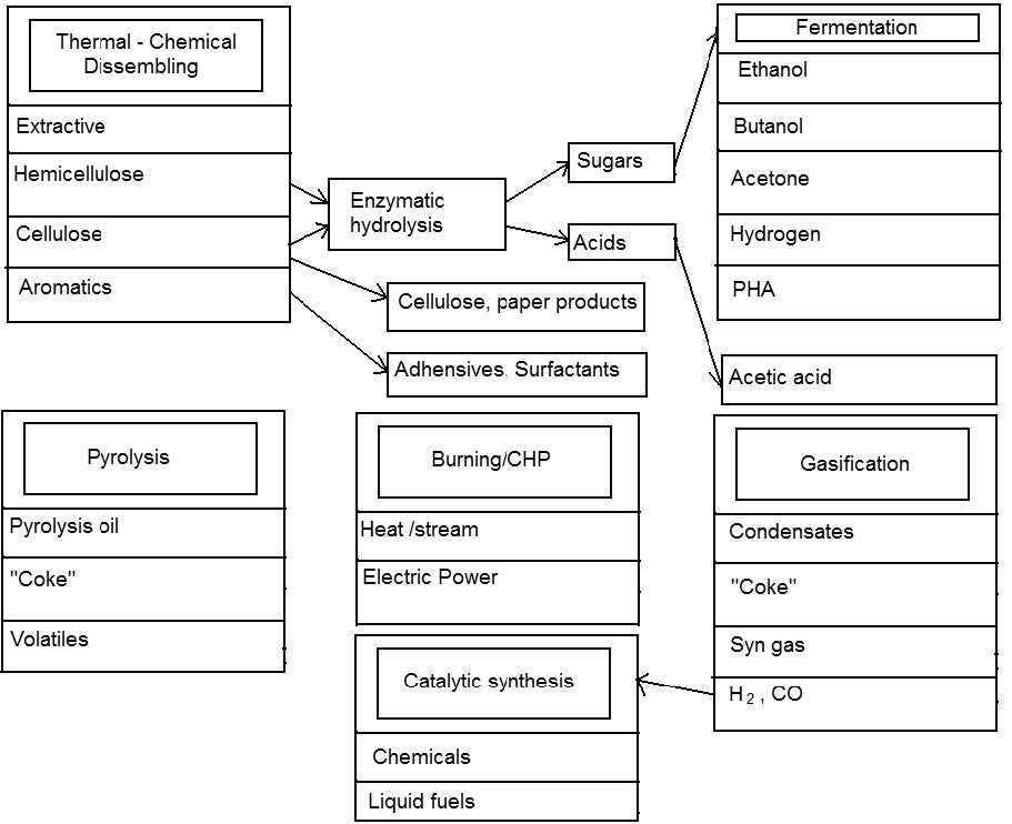
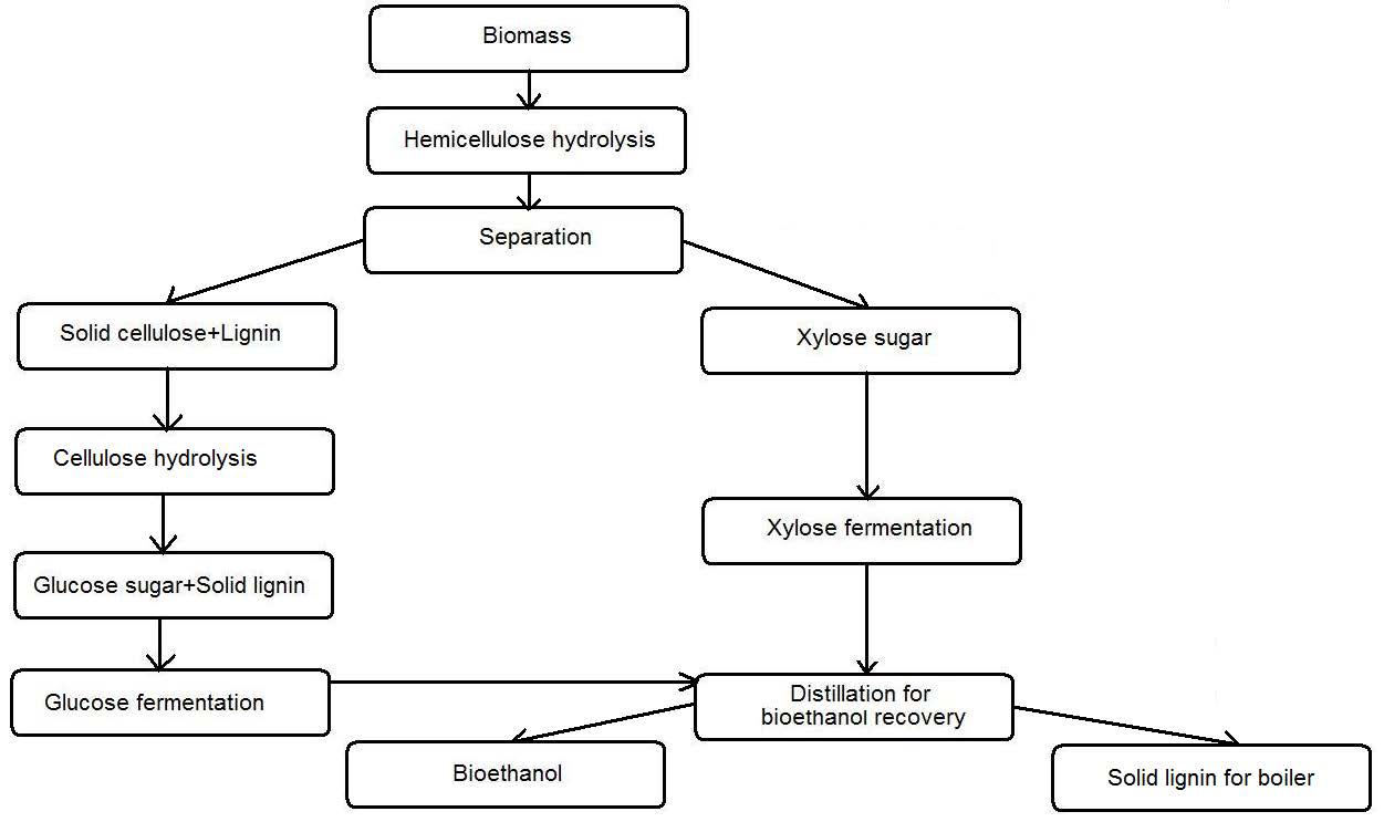
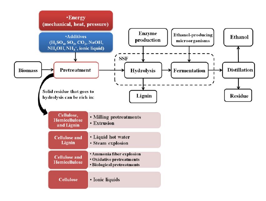
    [162] Silva AS, Teixeira RSS, Moutta RO, et al. (2013) Sugarcane and Woody Biomass Pretreatments for Ethanol Production. Chapter 3 In: Sustainable Degradation of Lignocellulosic Biomass - Techniques, Applications and Commercialization. Edited by Anuj K. Chandel and Silvio Silvério da Silva. InTech Eds. 42pp.
    [163] Fatehi Pedram (2013) Production of Biofuels from Cellulose of Woody Biomass. Chapter 3 In: Cellulose - Biomass Conversion. Edited by Theo van de Ven and John Kadla, InTech Eds. Available from: http://www.intechopen.com/books/cellulose-biomass-conversion/production-of-biofuels-from-cellulose-of-woody-biomass.
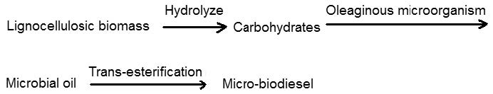
    [164] Dai CC, Tao J, Wang Y, et al. (2010) Research advance and superiority of microdiesel production with biowastes. Afr J Microbiol Res 4: 977-983.
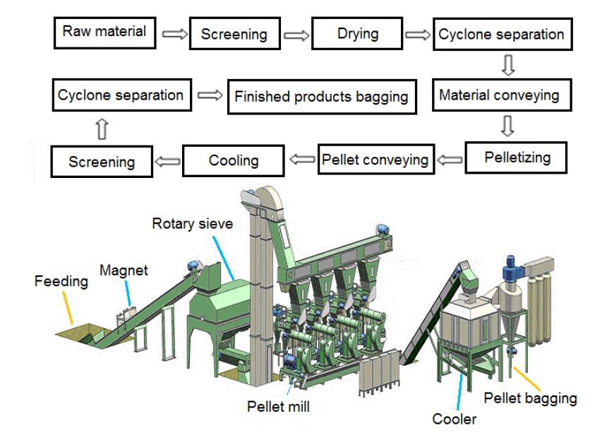
    [165] Huang J (2015) Pellet Plant Process Flow Chart: Gemco Energy. Available from: http://www.biomass-energy.org/blog/pellet-plant-process-flow-chart.html.
    [166] 
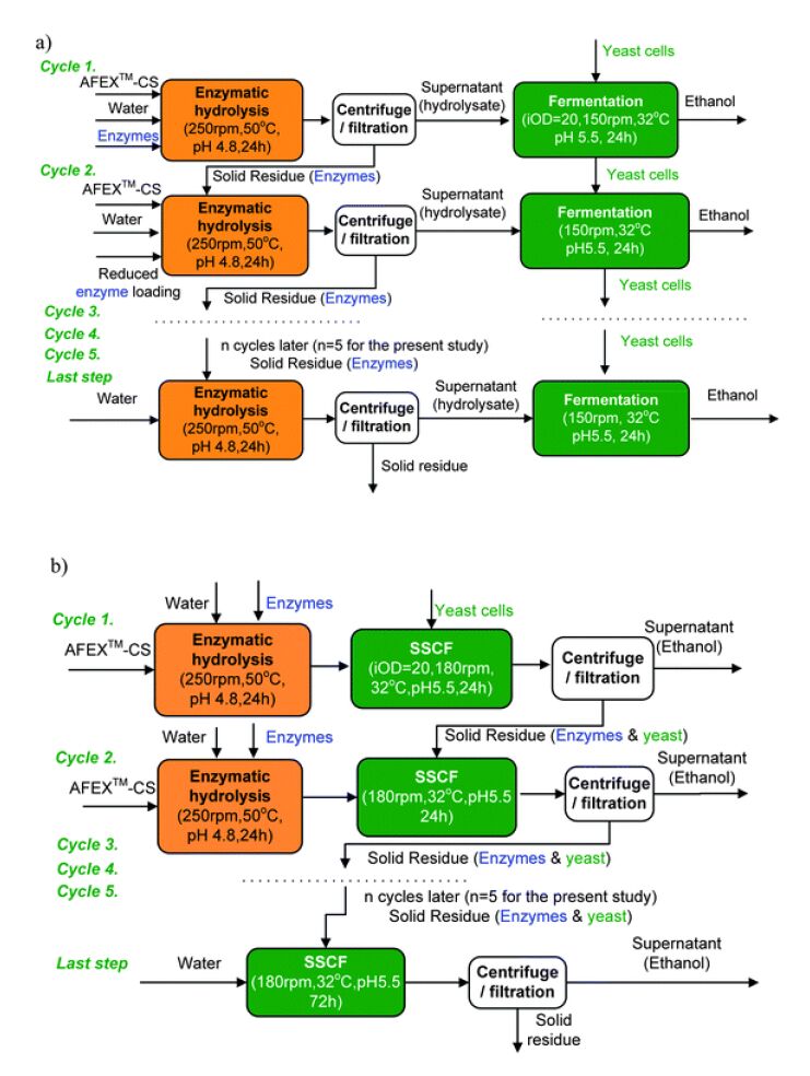
Jin M, Gunawan C, Uppugundla N, et al. (2012) A novel integrated biological process for cellulosic ethanol production featuring high ethanol productivity, enzyme recycling and yeast cells reuse. Energ Environ Sci 5: 7168-7175. doi: 10.1039/c2ee03058f
  • This article has been cited by:

    1. Konstantinos Giannakou, Maria Kyprianidou, Margarita Christofi, Anastasios Kalatzis, Georgia Fakonti, Mandatory COVID-19 Vaccination for Healthcare Professionals and Its Association With General Vaccination Knowledge: A Nationwide Cross-Sectional Survey in Cyprus, 2022, 10, 2296-2565, 10.3389/fpubh.2022.897526
    2. Lulla Opatowski, Laura Temime, Contributions of modelling for the control of COVID-19 nosocomial transmission, 2022, 41, 23525568, 101054, 10.1016/j.accpm.2022.101054
    3. Wenyu Chen, Ming Yao, Liang Dong, Pingyang Shao, Ye Zhang, Binjie Fu, The application framework of big data technology during the COVID-19 pandemic in China, 2022, 150, 0950-2688, 10.1017/S0950268822000577
    4. Jordana Vaz Hendler, Patricia Miranda do Lago, Gabriel Cardozo Müller, João Carlos Santana, Jefferson Pedro Piva, Liane Esteves Daudt, Risk factors for severe COVID-19 infection in Brazilian children, 2021, 25, 14138670, 101650, 10.1016/j.bjid.2021.101650
    5. Tom Dudding, Sadiyah Sheikh, Florence Gregson, Jennifer Haworth, Simon Haworth, Barry G. Main, Andrew J. Shrimpton, Fergus W. Hamilton, Anthony J. Ireland, Nick A. Maskell, Jonathan P. Reid, Bryan R. Bzdek, Mark Gormley, Markus Metsälä, A clinical observational analysis of aerosol emissions from dental procedures, 2022, 17, 1932-6203, e0265076, 10.1371/journal.pone.0265076
    6. David Moreno-Martos, Sean Foley, Benjamin Parcell, Dumitru Trucu, Raluca Eftimie, A computational investigation of COVID-19 transmission inside hospital wards and associated costs, 2022, 19, 1551-0018, 6504, 10.3934/mbe.2022306
    7. Meghann Gallouche, Caroline Landelle, Sylvie Larrat, Aurélie Truffot, Jean-Luc Bosson, Alban Caporossi, Towards real-time monitoring of COVID-19 nosocomial clusters using SARS-CoV-2 genomes in a university hospital of the French Alps, 2023, 26669919, 104650, 10.1016/j.idnow.2023.104650
    8. F. McAndrew, R.G. Abeysuriya, R. Sacks-Davis, M. Sammann, D.M. Lister, D. West, S.S. Majumdar, N. Scott, Admission screening testing of patients and staff N95 respirators are cost-effective in reducing COVID-19 hospital-acquired infections, 2024, 152, 01956701, 81, 10.1016/j.jhin.2024.06.015
    9. Sreejita Ghosh, Dibyajit Lahiri, Moupriya Nag, Rina Rani Ray, Debasmita Bhattacharya, 2024, Chapter 7, 978-981-99-9461-8, 145, 10.1007/978-981-99-9462-5_7
    10. D.R.M. Smith, S. Chervet, T. Pinettes, G. Shirreff, S. Jijón, A. Oodally, K. Jean, L. Opatowski, S. Kernéis, L. Temime, How have mathematical models contributed to understanding the transmission and control of SARS-CoV-2 in healthcare settings? A systematic search and review, 2023, 141, 01956701, 132, 10.1016/j.jhin.2023.07.028
    11. George Shirreff, Anne C.M. Thiébaut, Bich-Tram Huynh, Guillaume Chelius, Antoine Fraboulet, Didier Guillemot, Lulla Opatowski, Laura Temime, Hospital population density and risk of respiratory infection: is close contact density dependent?, 2024, 17554365, 100807, 10.1016/j.epidem.2024.100807
  • Reader Comments
  • © 2016 the Author(s), licensee AIMS Press. This is an open access article distributed under the terms of the Creative Commons Attribution License (http://creativecommons.org/licenses/by/4.0)
通讯作者: 陈斌, bchen63@163.com
  • 1. 

    沈阳化工大学材料科学与工程学院 沈阳 110142

  1. 本站搜索
  2. 百度学术搜索
  3. 万方数据库搜索
  4. CNKI搜索

Metrics

Article views(9080) PDF downloads(1390) Cited by(17)

Figures and Tables

Figures(7)  /  Tables(10)

/

DownLoad:  Full-Size Img  PowerPoint
Return
Return

Catalog